This rendered site is an archived version of the changes last made by Beck, minus some proprietary content from private repos — Visit live site

  • Documentation
    • About ​ValidMind
    • Get Started
    • Guides
    • Support

    • ValidMind Library
    • Python API
    • Public REST API

    • Training Courses

On this page

  • Prerequisites
  • Setting up
    • Initialize the ValidMind Library
    • Import sample dataset
    • Identify qualitative tests
    • Initialize the ValidMind dataset
  • Running tests on datasets
    • Run tabular data tests
    • Utilize test output
  • Documenting test results
    • Run and log multiple tests
    • Run and log an individual test
  • Running model evaluation tests
    • Train simple logistic regression model
    • Initialize ValidMind datasets
    • Initialize a ValidMind model
    • Run the model evaluation tests
  • In summary
  • Next steps
    • Integrate custom tests
  • Edit this page
  • Report an issue

ValidMind for development 2 — Start the development process

Learn how to use ValidMind for your end-to-end documentation process with our series of four introductory notebooks. In this second notebook, you'll run tests and investigate results, then add the results or evidence to your documentation.

You'll become familiar with the individual tests available in ValidMind, as well as how to run them and change parameters as necessary. Using ValidMind's repository of individual tests as building blocks helps you ensure that a record (model) is being built appropriately.

For a full list of out-of-the-box tests and descriptions, use the interactive ValidMind test sandbox.

Learn by doing

Our course tailor-made for developers new to ValidMind combines this series of notebooks with more a more in-depth introduction to the ValidMind Platform — Developer Fundamentals

Prerequisites

In order to log test results or evidence to your documentation with this notebook, you'll need to first have:

Need help with the above steps?

Refer to the first notebook in this series: 1 — Set up the ValidMind Library

Setting up

Initialize the ValidMind Library

First, let's connect up the ValidMind Library to our model we previously registered in the ValidMind Platform:

  1. On the left sidebar that appears for your model, select Getting Started and select Development from the Document drop-down menu.

  2. Click Copy snippet to clipboard.

  3. Next, load your model identifier credentials from an .env file or replace the placeholder with your own code snippet:

# Make sure the ValidMind Library is installed

%pip install -q validmind

# Load your model identifier credentials from an `.env` file

%load_ext dotenv
%dotenv .env

# Or replace with your code snippet

import validmind as vm

vm.init(
    # api_host="...",
    # api_key="...",
    # api_secret="...",
    # model="...",
    document="documentation",
)
Note: you may need to restart the kernel to use updated packages.
2026-07-31 16:39:18,470 - INFO(validmind.api_client): 🎉 Connected to ValidMind!
📊 Model: [ValidMind Academy] Model development (ID: cmalgf3qi02ce199qm3rdkl46)
📁 Document Type: model_documentation

Import sample dataset

Then, let's import the public Bank Customer Churn Prediction dataset from Kaggle.

In our below example, note that:

  • The target column, Exited has a value of 1 when a customer has churned and 0 otherwise.
  • The ValidMind Library provides a wrapper to automatically load the dataset as a Pandas DataFrame object. A Pandas Dataframe is a two-dimensional tabular data structure that makes use of rows and columns.
from validmind.datasets.classification import customer_churn as demo_dataset

print(
    f"Loaded demo dataset with: \n\n\t• Target column: '{demo_dataset.target_column}' \n\t• Class labels: {demo_dataset.class_labels}"
)

raw_df = demo_dataset.load_data()
raw_df.head()
Loaded demo dataset with: 

    • Target column: 'Exited' 
    • Class labels: {'0': 'Did not exit', '1': 'Exited'}
CreditScore Geography Gender Age Tenure Balance NumOfProducts HasCrCard IsActiveMember EstimatedSalary Exited
0 619 France Female 42 2 0.00 1 1 1 101348.88 1
1 608 Spain Female 41 1 83807.86 1 0 1 112542.58 0
2 502 France Female 42 8 159660.80 3 1 0 113931.57 1
3 699 France Female 39 1 0.00 2 0 0 93826.63 0
4 850 Spain Female 43 2 125510.82 1 1 1 79084.10 0

Identify qualitative tests

Next, let's say we want to do some data quality assessments by running a few individual tests.

Use the vm.tests.list_tests() function introduced by the first notebook in this series in combination with vm.tests.list_tags() and vm.tests.list_tasks() to find which prebuilt tests are relevant for data quality assessment:

  • tasks represent the kind of modeling task associated with a test. Here we'll focus on classification tasks.
  • tags are free-form descriptions providing more details about the test, for example, what category the test falls into. Here we'll focus on the data_quality tag.
# Get the list of available task types
sorted(vm.tests.list_tasks())
['classification',
 'clustering',
 'data_validation',
 'feature_extraction',
 'monitoring',
 'nlp',
 'regression',
 'residual_analysis',
 'text_classification',
 'text_generation',
 'text_qa',
 'text_summarization',
 'time_series_forecasting',
 'visualization']
# Get the list of available tags
sorted(vm.tests.list_tags())
['AUC',
 'analysis',
 'anomaly',
 'anomaly_detection',
 'bias_and_fairness',
 'binary_classification',
 'calibration',
 'categorical_data',
 'classification',
 'classification_metrics',
 'clustering',
 'correlation',
 'credit_risk',
 'data_analysis',
 'data_distribution',
 'data_quality',
 'data_validation',
 'descriptive_statistics',
 'dimensionality_reduction',
 'distribution',
 'embeddings',
 'feature_importance',
 'feature_selection',
 'few_shot',
 'forecasting',
 'frequency_analysis',
 'kmeans',
 'linear_regression',
 'llm',
 'logistic_regression',
 'metadata',
 'model_comparison',
 'model_diagnosis',
 'model_explainability',
 'model_interpretation',
 'model_performance',
 'model_predictions',
 'model_selection',
 'model_training',
 'model_validation',
 'multiclass_classification',
 'nlp',
 'normality',
 'numerical_data',
 'outlier',
 'outliers',
 'qualitative',
 'rag_performance',
 'ragas',
 'regression',
 'retrieval_performance',
 'scorecard',
 'seasonality',
 'senstivity_analysis',
 'sklearn',
 'stationarity',
 'statistical_test',
 'statistics',
 'statsmodels',
 'tabular_data',
 'text_data',
 'threshold_optimization',
 'time_series_data',
 'unit_root_test',
 'visualization',
 'zero_shot']

You can pass tags and tasks as parameters to the vm.tests.list_tests() function to filter the tests based on the tags and task types.

For example, to find tests related to tabular data quality for classification models, you can call list_tests() like this:

vm.tests.list_tests(task="classification", tags=["tabular_data", "data_quality"])
ID Name Description Has Figure Has Table Required Inputs Params Tags Tasks
validmind.data_validation.ClassImbalance Class Imbalance Evaluates and quantifies class distribution imbalance in a dataset used by a machine learning model.... True True ['dataset'] {'min_percent_threshold': {'type': 'int', 'default': 10}} ['tabular_data', 'binary_classification', 'multiclass_classification', 'data_quality'] ['classification']
validmind.data_validation.DescriptiveStatistics Descriptive Statistics Performs a detailed descriptive statistical analysis of both numerical and categorical data within a model's... False True ['dataset'] {} ['tabular_data', 'time_series_data', 'data_quality'] ['classification', 'regression']
validmind.data_validation.Duplicates Duplicates Tests dataset for duplicate entries, ensuring model reliability via data quality verification.... False True ['dataset'] {'min_threshold': {'type': '_empty', 'default': 1}} ['tabular_data', 'data_quality', 'text_data'] ['classification', 'regression']
validmind.data_validation.HighCardinality High Cardinality Assesses the number of unique values in categorical columns to detect high cardinality and potential overfitting.... False True ['dataset'] {'num_threshold': {'type': 'int', 'default': 100}, 'percent_threshold': {'type': 'float', 'default': 0.1}, 'threshold_type': {'type': 'str', 'default': 'percent'}} ['tabular_data', 'data_quality', 'categorical_data'] ['classification', 'regression']
validmind.data_validation.HighPearsonCorrelation High Pearson Correlation Identifies highly correlated feature pairs in a dataset suggesting feature redundancy or multicollinearity.... False True ['dataset'] {'max_threshold': {'type': 'float', 'default': 0.3}, 'top_n_correlations': {'type': 'int', 'default': 10}, 'feature_columns': {'type': 'list', 'default': None}} ['tabular_data', 'data_quality', 'correlation'] ['classification', 'regression']
validmind.data_validation.MissingValues Missing Values Evaluates dataset quality by ensuring missing value percentage across all features does not exceed a set threshold.... False True ['dataset'] {'min_percentage_threshold': {'type': 'float', 'default': 1.0}} ['tabular_data', 'data_quality'] ['classification', 'regression']
validmind.data_validation.MissingValuesBarPlot Missing Values Bar Plot Assesses the percentage and distribution of missing values in the dataset via a bar plot, with emphasis on... True False ['dataset'] {'threshold': {'type': 'int', 'default': 80}, 'fig_height': {'type': 'int', 'default': 600}} ['tabular_data', 'data_quality', 'visualization'] ['classification', 'regression']
validmind.data_validation.Skewness Skewness Evaluates the skewness of numerical data in a dataset to check against a defined threshold, aiming to ensure data... False True ['dataset'] {'max_threshold': {'type': '_empty', 'default': 1}} ['data_quality', 'tabular_data'] ['classification', 'regression']
validmind.plots.BoxPlot Box Plot Generates customizable box plots for numerical features in a dataset with optional grouping using Plotly.... True False ['dataset'] {'columns': {'type': 'Optional', 'default': None}, 'group_by': {'type': 'Optional', 'default': None}, 'width': {'type': 'int', 'default': 1800}, 'height': {'type': 'int', 'default': 1200}, 'colors': {'type': 'Optional', 'default': None}, 'show_outliers': {'type': 'bool', 'default': True}, 'title_prefix': {'type': 'str', 'default': 'Box Plot of'}} ['tabular_data', 'visualization', 'data_quality'] ['classification', 'regression', 'clustering']
validmind.plots.HistogramPlot Histogram Plot Generates customizable histogram plots for numerical features in a dataset using Plotly.... True False ['dataset'] {'columns': {'type': 'Optional', 'default': None}, 'bins': {'type': 'Union', 'default': 30}, 'color': {'type': 'str', 'default': 'steelblue'}, 'opacity': {'type': 'float', 'default': 0.7}, 'show_kde': {'type': 'bool', 'default': True}, 'normalize': {'type': 'bool', 'default': False}, 'log_scale': {'type': 'bool', 'default': False}, 'title_prefix': {'type': 'str', 'default': 'Histogram of'}, 'width': {'type': 'int', 'default': 1200}, 'height': {'type': 'int', 'default': 800}, 'n_cols': {'type': 'int', 'default': 2}, 'vertical_spacing': {'type': 'float', 'default': 0.15}, 'horizontal_spacing': {'type': 'float', 'default': 0.1}} ['tabular_data', 'visualization', 'data_quality'] ['classification', 'regression', 'clustering']
validmind.stats.DescriptiveStats Descriptive Stats Provides comprehensive descriptive statistics for numerical features in a dataset.... False True ['dataset'] {'columns': {'type': 'Optional', 'default': None}, 'include_advanced': {'type': 'bool', 'default': True}, 'confidence_level': {'type': 'float', 'default': 0.95}} ['tabular_data', 'statistics', 'data_quality'] ['classification', 'regression', 'clustering']
Want to learn more about navigating ValidMind tests?

Refer to our notebook outlining the utilities available for viewing and understanding available ValidMind tests: Explore tests

Initialize the ValidMind dataset

With the individual tests we want to run identified, the next step is to connect your data with a ValidMind Dataset object. This step is always necessary every time you want to connect a dataset to documentation and produce test results through ValidMind, but you only need to do it once per dataset.

Initialize a ValidMind dataset object using the init_dataset function from the ValidMind (vm) module. For this example, we'll pass in the following arguments:

  • dataset — The raw dataset that you want to provide as input to tests.
  • input_id — A unique identifier that allows tracking what inputs are used when running each individual test.
  • target_column — A required argument if tests require access to true values. This is the name of the target column in the dataset.
# vm_raw_dataset is now a VMDataset object that you can pass to any ValidMind test
vm_raw_dataset = vm.init_dataset(
    dataset=raw_df,
    input_id="raw_dataset",
    target_column="Exited",
)

Running tests on datasets

Now that we know how to initialize a ValidMind dataset object, we're ready to run some tests!

You run individual tests by calling the run_test function provided by the validmind.tests module. For the examples below, we'll pass in the following arguments:

  • test_id — The ID of the test to run, as seen in the ID column when you run list_tests.
  • params — A dictionary of parameters for the test. These will override any default_params set in the test definition.

Run tabular data tests

The inputs expected by a test can also be found in the test definition — let's take validmind.data_validation.DescriptiveStatistics as an example.

Note that the output of the describe_test() function below shows that this test expects a dataset as input:

vm.tests.describe_test("validmind.data_validation.DescriptiveStatistics")
▶ Test: Descriptive Statistics ('validmind.data_validation.DescriptiveStatistics')

Descriptive Statistics

Performs a detailed descriptive statistical analysis of both numerical and categorical data within a model's dataset.

Purpose

The purpose of the Descriptive Statistics metric is to provide a comprehensive summary of both numerical and categorical data within a dataset. This involves statistics such as count, mean, standard deviation, minimum and maximum values for numerical data. For categorical data, it calculates the count, number of unique values, most common value and its frequency, and the proportion of the most frequent value relative to the total. The goal is to visualize the overall distribution of the variables in the dataset, aiding in understanding the model's behavior and predicting its performance.

Test Mechanism

The testing mechanism utilizes two in-built functions of pandas dataframes: describe() for numerical fields and value_counts() for categorical fields. The describe() function pulls out several summary statistics, while value_counts() accounts for unique values. The resulting data is formatted into two distinct tables, one for numerical and another for categorical variable summaries. These tables provide a clear summary of the main characteristics of the variables, which can be instrumental in assessing the model's performance.

Signs of High Risk

  • Skewed data or significant outliers can represent high risk. For numerical data, this may be reflected via a significant difference between the mean and median (50% percentile).
  • For categorical data, a lack of diversity (low count of unique values), or overdominance of a single category (high frequency of the top value) can indicate high risk.

Strengths

  • Provides a comprehensive summary of the dataset, shedding light on the distribution and characteristics of the variables under consideration.
  • It is a versatile and robust method, applicable to both numerical and categorical data.
  • Helps highlight crucial anomalies such as outliers, extreme skewness, or lack of diversity, which are vital in understanding model behavior during testing and validation.

Limitations

  • While this metric offers a high-level overview of the data, it may fail to detect subtle correlations or complex patterns.
  • Does not offer any insights on the relationship between variables.
  • Alone, descriptive statistics cannot be used to infer properties about future unseen data.
  • Should be used in conjunction with other statistical tests to provide a comprehensive understanding of the model's data.

Required Inputs: dataset

Parameters:

Parameter Default Value

How to Run:

Code:

        
import validmind as vm

# inputs dictionary maps your inputs to the expected input names
# keys are the expected input names and values are the actual inputs
# values may be string input_ids or the actual VMDataset or VMModel objects
inputs = {
    "dataset": "my_vm_dataset"
}
params = {}

# to run and view the result of this test, run the following code:
result = vm.tests.run_test(
  "validmind.data_validation.DescriptiveStatistics", inputs=inputs, params=params
)

# To see the result of the test, ensure that you have called `vm.init()` and then run:
result.log()
    

Now, let's run a few tests to assess the quality of the dataset:

result = vm.tests.run_test(
    test_id="validmind.data_validation.DescriptiveStatistics",
    inputs={"dataset": vm_raw_dataset},
)

Descriptive Statistics

The Descriptive Statistics test evaluates the distributional characteristics of numerical and categorical variables in the dataset. The results summarize central tendency, dispersion, percentile structure, and range for eight numerical variables, alongside category counts, unique-value counts, and dominant-category frequencies for two categorical variables. All reported variables have a count of 8,000 observations, and the tables show how values are distributed across customer attributes, account characteristics, and binary indicators.

Key insights:

  • Balance shows a zero-heavy distribution: Balance has a minimum of 0, a 25th percentile of 0, and a median of 97,264, indicating that at least one quarter of observations are at zero while the remaining distribution extends to a maximum of 250,898. The mean of 76,434.10 is below the median, consistent with concentration at lower values.

  • EstimatedSalary is broadly dispersed: EstimatedSalary ranges from 12 to 199,992, with a mean of 99,790.19 and median of 99,505. The 25th and 75th percentiles of 50,857 and 149,216, together with a standard deviation of 57,520.51, indicate a wide spread across the observed salary distribution.

  • CreditScore and Age are centered near medians: CreditScore has a mean of 650.16 and median of 652, while Age has a mean of 38.95 and median of 37. The close alignment between means and medians indicates relatively stable central tendency for these variables within their observed ranges.

  • Product holdings are concentrated at lower counts: NumOfProducts has a median of 1, a 75th percentile of 2, and a maximum of 4, with a mean of 1.53. This indicates concentration in the lower product-count categories.

  • Binary indicators are unevenly distributed: HasCrCard has a mean of 0.7026, indicating that the value 1 occurs more frequently than 0, while IsActiveMember has a mean of 0.5199, indicating a more balanced split. For both variables, the median and upper percentiles are 1.

  • Geography is moderately concentrated; Gender is near-balanced: Geography contains 3 unique values, with France as the top category at 4,010 observations (50.12%). Gender contains 2 unique values, with Male as the top category at 4,396 observations (54.95%), indicating a modest majority rather than a dominant concentration.

The results show full observation counts across all reported variables and a mix of distribution shapes across the dataset. The most distinct numerical feature is Balance, where zero values are concentrated in the lower quartile while the upper range remains wide; EstimatedSalary also exhibits substantial dispersion across its range. Other variables, including CreditScore, Age, product counts, and the binary and categorical fields, display more contained distributions, with moderate category concentration in Geography and a near-balanced split in Gender.

Tables

Numerical Variables

Name Count Mean Std Min 25% 50% 75% 90% 95% Max
CreditScore 8000.0 650.1596 96.8462 350.0 583.0 652.0 717.0 778.0 813.0 850.0
Age 8000.0 38.9489 10.4590 18.0 32.0 37.0 44.0 53.0 60.0 92.0
Tenure 8000.0 5.0339 2.8853 0.0 3.0 5.0 8.0 9.0 9.0 10.0
Balance 8000.0 76434.0965 62612.2513 0.0 0.0 97264.0 128045.0 149545.0 162488.0 250898.0
NumOfProducts 8000.0 1.5325 0.5805 1.0 1.0 1.0 2.0 2.0 2.0 4.0
HasCrCard 8000.0 0.7026 0.4571 0.0 0.0 1.0 1.0 1.0 1.0 1.0
IsActiveMember 8000.0 0.5199 0.4996 0.0 0.0 1.0 1.0 1.0 1.0 1.0
EstimatedSalary 8000.0 99790.1880 57520.5089 12.0 50857.0 99505.0 149216.0 179486.0 189997.0 199992.0

Categorical Variables

Name Count Number of Unique Values Top Value Top Value Frequency Top Value Frequency %
Geography 8000.0 3.0 France 4010.0 50.12
Gender 8000.0 2.0 Male 4396.0 54.95
result2 = vm.tests.run_test(
    test_id="validmind.data_validation.ClassImbalance",
    inputs={"dataset": vm_raw_dataset},
    params={"min_percent_threshold": 30},
)

❌ Class Imbalance

The Class Imbalance test evaluates the distribution of target classes in the dataset by measuring each class’s share of total records against a defined minimum percentage threshold. In this run, the target variable Exited is summarized across two classes with a threshold of 30%. The results table and bar chart show that class Exited = 0 represents 79.80% of rows and is marked as Pass, while class Exited = 1 represents 20.20% of rows and is marked as Fail.

Key insights:

  • Majority class dominates distribution: Exited = 0 accounts for 79.80% of the dataset, making it the predominant class in the target distribution.

  • Minority class falls below threshold: Exited = 1 represents 20.20% of rows, which is below the configured 30% minimum threshold and is therefore marked as Fail.

  • Pass/fail outcome differs by class: The test produces a mixed result across classes, with the majority class passing the threshold criterion and the minority class failing it.

The observed class distribution is uneven, with a large concentration in Exited = 0 and a smaller share in Exited = 1. Under the configured 30% threshold, only the majority class satisfies the minimum representation requirement, while the minority class does not. Collectively, these results indicate that the target distribution contains a threshold-defined class imbalance.

Parameters:

{
  "min_percent_threshold": 30
}
            

Tables

Exited Class Imbalance

Exited Percentage of Rows (%) Pass/Fail
0 79.80% Pass
1 20.20% Fail

Figures

ValidMind Figure validmind.data_validation.ClassImbalance:7f94

The output above shows that the validmind.data_validation.ClassImbalance test did not pass according to the value we set for min_percent_threshold.

To address this issue, we'll re-run the test on some processed data. In this case let's apply a very simple rebalancing technique to the dataset:

import pandas as pd

raw_copy_df = raw_df.sample(frac=1)  # Create a copy of the raw dataset

# Create a balanced dataset with the same number of exited and not exited customers
exited_df = raw_copy_df.loc[raw_copy_df["Exited"] == 1]
not_exited_df = raw_copy_df.loc[raw_copy_df["Exited"] == 0].sample(n=exited_df.shape[0])

balanced_raw_df = pd.concat([exited_df, not_exited_df])
balanced_raw_df = balanced_raw_df.sample(frac=1, random_state=42)

With this new balanced dataset, you can re-run the individual test to see if it now passes the class imbalance test requirement.

As this is technically a different dataset, remember to first initialize a new ValidMind Dataset object to pass in as input as required by run_test():

# Register new data and now 'balanced_raw_dataset' is the new dataset object of interest
vm_balanced_raw_dataset = vm.init_dataset(
    dataset=balanced_raw_df,
    input_id="balanced_raw_dataset",
    target_column="Exited",
)
# Pass the initialized `balanced_raw_dataset` as input into the test run
result = vm.tests.run_test(
    test_id="validmind.data_validation.ClassImbalance",
    inputs={"dataset": vm_balanced_raw_dataset},
    params={"min_percent_threshold": 30},
)

✅ Class Imbalance

The Class Imbalance test evaluates the distribution of target classes in the dataset by measuring the percentage of records in each class and comparing those percentages with the configured minimum threshold. In this run, the target variable Exited is shown across two classes, 0 and 1, with the table and bar chart both indicating an equal class share of 50.00% for each class. The test was executed using a minimum percentage threshold of 30, and the result table reports a pass/fail outcome for each class.

Key insights:

  • Classes are evenly split: The Exited target is distributed evenly across the two observed classes, with 50.00% of rows in class 0 and 50.00% in class 1.
  • Both classes exceed threshold: Each class is above the configured 30% minimum percentage threshold, and both classes are marked as Pass.
  • No under-represented target class observed: The result table does not show any class below the threshold, and the plot confirms equal bar heights for both target categories.

The observed target distribution is fully balanced between the two Exited classes, with identical representation at 50.00% each. Relative to the configured 30% threshold, both classes satisfy the test criterion and no class-level imbalance is indicated by this result.

Parameters:

{
  "min_percent_threshold": 30
}
            

Tables

Exited Class Imbalance

Exited Percentage of Rows (%) Pass/Fail
0 50.00% Pass
1 50.00% Pass

Figures

ValidMind Figure validmind.data_validation.ClassImbalance:aa24

Utilize test output

You can utilize the output from a ValidMind test for further use, for example, if you want to remove highly correlated features. Removing highly correlated features helps make the model simpler, more stable, and easier to understand.

Below we demonstrate how to retrieve the list of features with the highest correlation coefficients and use them to reduce the final list of features for modeling.

First, we'll run validmind.data_validation.HighPearsonCorrelation with the balanced_raw_dataset we initialized previously as input as is for comparison with later runs:

corr_result = vm.tests.run_test(
    test_id="validmind.data_validation.HighPearsonCorrelation",
    params={"max_threshold": 0.3},
    inputs={"dataset": vm_balanced_raw_dataset},
)

❌ High Pearson Correlation

The High Pearson Correlation test evaluates pairwise linear relationships among features to identify correlations that may indicate redundancy or multicollinearity. The result table reports the top 10 feature pairs ranked by Pearson correlation coefficient, along with Pass/Fail status based on the configured absolute correlation threshold of 0.3. Observed coefficients range from -0.1923 to 0.3512, and only one pair exceeds the threshold. The strongest reported relationship is between Age and Exited, while the remaining listed pairs fall within the passing range.

Key insights:

  • Single threshold breach identified: The pair (Age, Exited) records the highest coefficient at 0.3512 and is the only result marked Fail, exceeding the configured threshold of 0.3.
  • Remaining correlations are limited in magnitude: The other nine reported feature pairs all pass the test, with absolute coefficients between 0.0349 and 0.1923, indicating weaker linear relationships within the reported set.
  • Largest negative relationship remains below threshold: The strongest negative coefficient is -0.1923 for (IsActiveMember, Exited), which remains below the threshold and is marked Pass.
  • Top reported relationships are concentrated near zero to low magnitude: Several listed pairs, including (Tenure, Exited) at -0.0368, (HasCrCard, IsActiveMember) at -0.0367, and (Age, Balance) at 0.0349, show correlations close to zero.

The reported correlation structure is dominated by low-magnitude pairwise linear relationships, with (Age, Exited) as the only feature pair exceeding the configured threshold. All other listed pairs remain within the passing range, including the strongest negative relationship. Overall, the table shows one flagged correlation and a broader set of comparatively weak linear associations among the top reported pairs.

Parameters:

{
  "max_threshold": 0.3
}
            

Tables

Columns Coefficient Pass/Fail
(Age, Exited) 0.3512 Fail
(IsActiveMember, Exited) -0.1923 Pass
(Balance, NumOfProducts) -0.1722 Pass
(Balance, Exited) 0.1414 Pass
(Tenure, IsActiveMember) -0.0590 Pass
(NumOfProducts, Exited) -0.0495 Pass
(NumOfProducts, IsActiveMember) 0.0418 Pass
(Tenure, Exited) -0.0368 Pass
(HasCrCard, IsActiveMember) -0.0367 Pass
(Age, Balance) 0.0349 Pass

The output above shows that the test did not pass according to the value we set for max_threshold.

corr_result is an object of type TestResult. We can inspect the result object to see what the test has produced:

print(type(corr_result))
print("Result ID: ", corr_result.result_id)
print("Params: ", corr_result.params)
print("Passed: ", corr_result.passed)
print("Tables: ", corr_result.tables)
<class 'validmind.vm_models.result.result.TestResult'>
Result ID:  validmind.data_validation.HighPearsonCorrelation
Params:  {'max_threshold': 0.3}
Passed:  False
Tables:  [ResultTable]

Let's remove the highly correlated features and create a new VM dataset object.

We'll begin by checking out the table in the result and extracting a list of features that failed the test:

# Extract table from `corr_result.tables`
features_df = corr_result.tables[0].data
features_df
Columns Coefficient Pass/Fail
0 (Age, Exited) 0.3512 Fail
1 (IsActiveMember, Exited) -0.1923 Pass
2 (Balance, NumOfProducts) -0.1722 Pass
3 (Balance, Exited) 0.1414 Pass
4 (Tenure, IsActiveMember) -0.0590 Pass
5 (NumOfProducts, Exited) -0.0495 Pass
6 (NumOfProducts, IsActiveMember) 0.0418 Pass
7 (Tenure, Exited) -0.0368 Pass
8 (HasCrCard, IsActiveMember) -0.0367 Pass
9 (Age, Balance) 0.0349 Pass
# Extract list of features that failed the test
high_correlation_features = features_df[features_df["Pass/Fail"] == "Fail"]["Columns"].tolist()
high_correlation_features
['(Age, Exited)']

Next, extract the feature names from the list of strings (example: (Age, Exited) > Age):

high_correlation_features = [feature.split(",")[0].strip("()") for feature in high_correlation_features]
high_correlation_features
['Age']

Now, it's time to re-initialize the dataset with the highly correlated features removed.

Note the use of a different input_id. This allows tracking the inputs used when running each individual test.

# Remove the highly correlated features from the dataset
balanced_raw_no_age_df = balanced_raw_df.drop(columns=high_correlation_features)

# Re-initialize the dataset object
vm_raw_dataset_preprocessed = vm.init_dataset(
    dataset=balanced_raw_no_age_df,
    input_id="raw_dataset_preprocessed",
    target_column="Exited",
)

Re-running the test with the reduced feature set should pass the test:

corr_result = vm.tests.run_test(
    test_id="validmind.data_validation.HighPearsonCorrelation",
    params={"max_threshold": 0.3},
    inputs={"dataset": vm_raw_dataset_preprocessed},
)

✅ High Pearson Correlation

The High Pearson Correlation test evaluates pairwise linear relationships among features to identify potentially redundant variables or multicollinearity. The result table lists the top feature pairs ranked by Pearson correlation coefficient, alongside Pass/Fail status based on the configured absolute threshold of 0.3. In this run, the reported coefficients range from -0.1923 to 0.1414 across the ten strongest observed pairs, and all listed relationships are marked as Pass.

Key insights:

  • No correlations exceed threshold: All reported absolute correlation coefficients are below the 0.3 threshold. Every listed feature pair is therefore classified as Pass in the test output.
  • Strongest observed relationship is modest: The largest absolute coefficient is -0.1923 for the pair (IsActiveMember, Exited). This indicates that the strongest linear association identified in the reported pairs remains limited in magnitude.
  • Top correlations are concentrated near zero: The remaining reported coefficients span from -0.1722 to 0.1414, with several values close to zero, including 0.0306, -0.0309, and -0.0367. This reflects generally weak pairwise linear dependence among the listed variables.
  • Both positive and negative associations appear: The output includes negative correlations such as (Balance, NumOfProducts) at -0.1722 and positive correlations such as (Balance, Exited) at 0.1414. The observed relationships are therefore mixed in direction, without any high-magnitude linear pair.

Overall, the reported correlation structure is weak across the top-ranked feature pairs in this test run. No listed feature pair breaches the configured threshold, and the highest absolute correlation remains below 0.2. Based on the reported output, the test does not identify strong pairwise linear dependence among the displayed variables.

Parameters:

{
  "max_threshold": 0.3
}
            

Tables

Columns Coefficient Pass/Fail
(IsActiveMember, Exited) -0.1923 Pass
(Balance, NumOfProducts) -0.1722 Pass
(Balance, Exited) 0.1414 Pass
(Tenure, IsActiveMember) -0.0590 Pass
(NumOfProducts, Exited) -0.0495 Pass
(NumOfProducts, IsActiveMember) 0.0418 Pass
(Tenure, Exited) -0.0368 Pass
(HasCrCard, IsActiveMember) -0.0367 Pass
(CreditScore, Exited) -0.0309 Pass
(Tenure, HasCrCard) 0.0306 Pass

You can also plot the correlation matrix to visualize the new correlation between features:

corr_result = vm.tests.run_test(
    test_id="validmind.data_validation.PearsonCorrelationMatrix",
    inputs={"dataset": vm_raw_dataset_preprocessed},
)

Pearson Correlation Matrix

The PearsonCorrelationMatrix test evaluates linear dependency between numerical variables in the dataset using pairwise Pearson correlation coefficients. The result is presented as a symmetric heat map covering CreditScore, Tenure, Balance, NumOfProducts, HasCrCard, IsActiveMember, EstimatedSalary, and Exited, with coefficient values ranging from -1 to 1 and diagonal values of 1.0. Off-diagonal correlations in this matrix are generally close to zero, with the largest observed magnitudes occurring in relationships involving Exited, Balance, NumOfProducts, and IsActiveMember.

Key insights:

  • No high pairwise correlations observed: All off-diagonal correlation coefficients remain well below the 0.70 absolute threshold highlighted by the test. The largest observed absolute correlation is 0.19.

  • Exited shows weak linear relationships: Exited has small correlations with the other numerical variables, with the largest magnitudes at -0.19 for IsActiveMember and 0.14 for Balance. Correlations with CreditScore (-0.03), Tenure (-0.04), NumOfProducts (-0.05), HasCrCard (-0.02), and EstimatedSalary (-0.0) are negligible.

  • Balance and NumOfProducts are mildly inversely related: The correlation between Balance and NumOfProducts is -0.17, representing one of the larger non-target pairwise relationships in the matrix, though still weak in magnitude.

  • Most predictor relationships are near zero: CreditScore, Tenure, HasCrCard, and EstimatedSalary exhibit correlations clustered around zero with the rest of the variables. This indicates limited linear association across most feature pairs in the dataset.

The correlation structure is sparse, with no material evidence of strong linear redundancy among the numerical variables included in the test. The most notable relationships are limited to weak associations involving Exited and a mild inverse relationship between Balance and NumOfProducts. Overall, the matrix indicates low pairwise linear dependence across the evaluated variables.

Figures

ValidMind Figure validmind.data_validation.PearsonCorrelationMatrix:2d34

Documenting test results

Now that we've done some analysis on two different datasets, we can use ValidMind to easily document why certain things were done to our raw data with testing to support it.

Every test result returned by the run_test() function has a .log() method that can be used to send the test results to the ValidMind Platform:

  • When using run_documentation_tests(), documentation sections will be automatically populated with the results of all tests registered in the documentation template.
  • When logging individual test results to the platform, you'll need to manually add those results to the desired section of the documentation.

To demonstrate how to add test results to your documentation, we'll populate the entire Data Preparation section of the documentation using the clean vm_raw_dataset_preprocessed dataset as input, and then document an additional individual result for the highly correlated dataset vm_balanced_raw_dataset.

Run and log multiple tests

run_documentation_tests() allows you to run multiple tests at once and automatically log the results to your documentation. Below, we'll run the tests using the previously initialized vm_raw_dataset_preprocessed as input — this will populate the entire Data Preparation section for every test that is part of the documentation template.

For this example, we'll pass in the following arguments:

  • inputs: Any inputs to be passed to the tests.
  • config: A dictionary <test_id>:<test_config> that allows configuring each test individually. Each test config requires the following:
    • params: Individual test parameters.
    • inputs: Individual test inputs. This overrides any inputs passed from the run_documentation_tests() function.

When including explicit configuration for individual tests, you'll need to specify the inputs even if they mirror what is included in your global configuration.

# Individual test config with inputs specified
test_config = {
    "validmind.data_validation.ClassImbalance": {
        "params": {"min_percent_threshold": 30},
        "inputs": {"dataset": vm_raw_dataset_preprocessed},
    },
    "validmind.data_validation.HighPearsonCorrelation": {
        "params": {"max_threshold": 0.3},
        "inputs": {"dataset": vm_raw_dataset_preprocessed},
    },
}

# Global test config
tests_suite = vm.run_documentation_tests(
    inputs={
        "dataset": vm_raw_dataset_preprocessed,
    },
    config=test_config,
    section=["data_preparation"],
)
Test suite complete!
26/26 (100.0%)

Test Suite Results: Binary Classification V2


Check out the updated documentation on ValidMind.

Template for binary classification models.

▶ Data Preparation

Data Preparation

▶ Test Result: Dataset Description (validmind.data_validation.DatasetDescription)

Dataset Description

The Dataset Description test evaluates the structure, completeness, and value cardinality of each dataset column. The results summarize 10 variables across numeric and categorical types, reporting count, missingness, and distinct-value statistics for each field. All listed columns contain 3,232 observed values, with separate columns showing the number and proportion of distinct values. The table also indicates the inferred data type for each variable, including five numeric fields and five categorical fields.

Key insights:

  • No missing values observed: All 10 variables report a missing count of 0 and a missing percentage of 0.0%, indicating complete population of the dataset fields included in the summary.

  • EstimatedSalary is fully unique: EstimatedSalary has 3,232 distinct values out of 3,232 observations, corresponding to a distinct proportion of 1.0, making it the highest-cardinality field in the dataset.

  • Balance also has high cardinality: Balance contains 2,210 distinct values, representing 68.38% of observations, which is materially higher than the distinctness observed in the other numeric variables except EstimatedSalary.

  • Most categorical fields are low-cardinality: Geography has 3 distinct values, while Gender, HasCrCard, IsActiveMember, and Exited each have 2 distinct values. These fields therefore exhibit very limited category counts relative to the dataset size.

  • Discrete numeric fields have limited value ranges: Tenure has 11 distinct values and NumOfProducts has 4 distinct values, indicating that these numeric variables take on a relatively small set of repeated values across the 3,232 records.

The dataset summary indicates complete coverage across all reported fields, with no missing observations in either numeric or categorical variables. Variable cardinality is heterogeneous: EstimatedSalary and Balance are the most granular fields, while several categorical variables and some numeric fields take only a small number of distinct values. Overall, the result provides a clear structural profile of the dataset, showing a mix of high-cardinality continuous-like variables and low-cardinality discrete variables.

Tables

Dataset Description

Name Type Count Missing Missing % Distinct Distinct %
CreditScore Numeric 3232.0 0 0.0 433 0.1340
Geography Categorical 3232.0 0 0.0 3 0.0009
Gender Categorical 3232.0 0 0.0 2 0.0006
Tenure Numeric 3232.0 0 0.0 11 0.0034
Balance Numeric 3232.0 0 0.0 2210 0.6838
NumOfProducts Numeric 3232.0 0 0.0 4 0.0012
HasCrCard Categorical 3232.0 0 0.0 2 0.0006
IsActiveMember Categorical 3232.0 0 0.0 2 0.0006
EstimatedSalary Numeric 3232.0 0 0.0 3232 1.0000
Exited Categorical 3232.0 0 0.0 2 0.0006
▶ Test Result: Class Imbalance (validmind.data_validation.ClassImbalance)

✅ Class Imbalance

The Class Imbalance test evaluates the distribution of target classes in a classification dataset. In this result, the target variable Exited is shown across two classes, with the table and bar chart reporting the percentage of rows associated with each class. Both class 0 and class 1 account for 50.00% of observations, and each is assessed against the configured minimum percentage threshold of 30%. The reported pass/fail status indicates that both classes pass the test.

Key insights:

  • Classes are evenly split: The Exited target is distributed equally across the two classes, with 50.00% of rows in class 0 and 50.00% in class 1.

  • All classes exceed threshold: The configured minimum percentage threshold is 30%, and both classes are 20 percentage points above this level.

  • No class-level failures observed: The pass/fail results show Pass for both target classes, indicating no underrepresented class under the applied test criterion.

The result shows a fully balanced observed class distribution for the Exited target under the configured Class Imbalance test. Each class represents half of the dataset and exceeds the 30% threshold, with no class flagged by the test. Collectively, the table and chart indicate no imbalance under this evaluation setup.

Parameters:

{
  "min_percent_threshold": 30
}
            

Tables

Exited Class Imbalance

Exited Percentage of Rows (%) Pass/Fail
0 50.00% Pass
1 50.00% Pass

Figures

ValidMind Figure validmind.data_validation.ClassImbalance:fb70
▶ Test Result: Duplicates (validmind.data_validation.Duplicates)

✅ Duplicates

The Duplicates test evaluates the dataset for exact duplicate rows to quantify redundancy in the data used for modeling. The result table reports both the count of duplicate rows and the corresponding share of total rows. In this run, the dataset contains 0 duplicate rows, representing 0.0% of all rows.

Key insights:

  • No duplicate rows detected: The test identified 0 duplicate rows in the dataset, indicating that no exact row-level repetitions were found.
  • Duplicate share is zero: The percentage of rows classified as duplicates is 0.0%, showing that duplicate incidence is absent in the tested data.

The test result indicates that exact row-level duplication was not present in the dataset at the time of evaluation. Both the absolute duplicate count and the duplicate percentage are zero, showing no observed redundancy under this test’s exact-match duplicate detection approach.

Tables

Duplicate Rows Results for Dataset

Number of Duplicates Percentage of Rows (%)
0 0.0
▶ Test Result: High Cardinality (validmind.data_validation.HighCardinality)

✅ High Cardinality

The High Cardinality test evaluates the number of unique values in categorical columns to identify categorical features with large counts of distinct values. The result table reports each categorical column alongside its number of distinct values, percentage of distinct values, and pass/fail outcome under the applied threshold. Two categorical columns were evaluated: Geography and Gender. Geography has 3 distinct values with 0.0928% distinctness, and Gender has 2 distinct values with 0.0619% distinctness; both columns passed the test.

Key insights:

  • All evaluated columns passed: Both categorical variables in scope, Geography and Gender, received a Pass result under the applied numeric threshold.
  • Low distinct counts observed: Geography contains 3 distinct values and Gender contains 2 distinct values, indicating limited category variation across the evaluated categorical features.
  • Distinctness percentages are minimal: The percentage of distinct values is 0.0928% for Geography and 0.0619% for Gender, with Geography marginally higher than Gender.

The test results show that the evaluated categorical columns did not exhibit high cardinality under the applied test criteria. Both features remained well below the threshold used for assessment, with low absolute and percentage distinct counts. Across the categorical variables included in the result, no failed high-cardinality cases were observed.

Tables

Column Number of Distinct Values Percentage of Distinct Values (%) Pass/Fail
Geography 3 0.0928 Pass
Gender 2 0.0619 Pass
▶ Test Result: Missing Values (validmind.data_validation.MissingValues)

✅ Missing Values

The Missing Values test evaluates dataset completeness by measuring the proportion of missing entries in each feature against the configured threshold. The result table reports the number and percentage of missing values for each column, together with a pass/fail status. In this run, all listed features show 0 missing values and 0.0% missingness, and each column receives a Pass result.

Key insights:

  • No missing values detected: All 10 evaluated columns report 0 missing values and 0.0% missingness.
  • All features passed the test: Every feature, including predictors and the target variable Exited, is marked Pass in the result table.
  • Missingness is uniformly absent: No variation in missing-value rates is present across the dataset; each column has the same observed missingness outcome of 0.0%.

The test result shows complete observed data coverage across all evaluated fields, with no missing entries recorded in any column. The absence of missingness is consistent across both input features and the target variable, and the pass/fail outcomes indicate that all columns remain within the specified missing-value threshold.

Tables

Column Number of Missing Values Percentage of Missing Values (%) Pass/Fail
CreditScore 0 0.0 Pass
Geography 0 0.0 Pass
Gender 0 0.0 Pass
Tenure 0 0.0 Pass
Balance 0 0.0 Pass
NumOfProducts 0 0.0 Pass
HasCrCard 0 0.0 Pass
IsActiveMember 0 0.0 Pass
EstimatedSalary 0 0.0 Pass
Exited 0 0.0 Pass
▶ Test Result: Skewness (validmind.data_validation.Skewness)

❌ Skewness

The Skewness test evaluates the asymmetry of numerical feature distributions by calculating skewness for each numeric column and comparing the result against the maximum threshold of 1. The results table reports skewness values and pass/fail outcomes for eight numerical columns in the dataset. Seven columns are marked as Pass, with skewness values ranging from -0.9018 to 0.1390, while one column is marked as Fail. The only failing feature is NumOfProducts, with a skewness value of 1.2444.

Key insights:

  • Single feature exceeds threshold: NumOfProducts is the only column that fails the test, with skewness of 1.2444, exceeding the threshold of 1.
  • Most features show limited asymmetry: Seven of eight numerical columns pass the test, with skewness values clustered near zero or remaining within the threshold bounds.
  • Largest negative skew remains within limit: HasCrCard has the most negative skewness at -0.9018, followed by Balance at -0.2849, and both remain classified as Pass.
  • Several variables are nearly symmetric: Exited has skewness of 0.0000, while Tenure and EstimatedSalary are also close to zero at 0.0086 and -0.0133 respectively.

The skewness assessment shows that distributional asymmetry is limited across most numerical inputs, with only one feature exceeding the defined threshold. The result is concentrated in NumOfProducts, while the remaining variables exhibit skewness values within the accepted range, including several that are effectively symmetric. Overall, the observed skewness profile is largely uniform apart from this isolated exception.

Tables

Skewness Results for Dataset

Column Skewness Pass/Fail
CreditScore -0.0928 Pass
Tenure 0.0086 Pass
Balance -0.2849 Pass
NumOfProducts 1.2444 Fail
HasCrCard -0.9018 Pass
IsActiveMember 0.1390 Pass
EstimatedSalary -0.0133 Pass
Exited 0.0000 Pass
▶ Test Result: Unique Rows (validmind.data_validation.UniqueRows)

❌ Unique Rows

The UniqueRows test evaluates data diversity by comparing the number and percentage of distinct values in each column against a prescribed threshold. The results are reported at the column level, showing the count of unique values, the corresponding percentage of unique values, and a pass/fail outcome for each feature. In this run, three columns passed the test and seven columns failed, with unique-value percentages ranging from 0.0619% to 100.0%.

Key insights:

  • Uniqueness is concentrated in numeric fields: EstimatedSalary shows 3,232 unique values and 100.0% uniqueness, Balance shows 2,210 unique values and 68.3787% uniqueness, and CreditScore shows 433 unique values and 13.3973% uniqueness. These are the only columns that passed the test.

  • Most columns have very low cardinality: Geography, Gender, Tenure, NumOfProducts, HasCrCard, IsActiveMember, and Exited all failed the test, with unique-value percentages between 0.0619% and 0.3403%. This indicates that distinct values are limited across most fields in the dataset.

  • Several variables are effectively binary: Gender, HasCrCard, IsActiveMember, and Exited each contain 2 unique values, corresponding to 0.0619% uniqueness. Their test outcomes are all Fail.

  • Categorical breadth varies across failed fields: Among the failing columns, Tenure has 11 unique values and 0.3403% uniqueness, NumOfProducts has 4 unique values and 0.1238%, and Geography has 3 unique values and 0.0928%. These values remain below the test threshold despite differing cardinalities.

The test results show a mixed uniqueness profile across the dataset, with passing results limited to CreditScore, Balance, and EstimatedSalary and failures concentrated in lower-cardinality columns. The strongest uniqueness is observed in EstimatedSalary and Balance, while multiple columns are binary or have only a small set of distinct values. Overall, the observed diversity is uneven across features, with most columns registering very low unique-value percentages under this test.

Tables

Column Number of Unique Values Percentage of Unique Values (%) Pass/Fail
CreditScore 433 13.3973 Pass
Geography 3 0.0928 Fail
Gender 2 0.0619 Fail
Tenure 11 0.3403 Fail
Balance 2210 68.3787 Pass
NumOfProducts 4 0.1238 Fail
HasCrCard 2 0.0619 Fail
IsActiveMember 2 0.0619 Fail
EstimatedSalary 3232 100.0000 Pass
Exited 2 0.0619 Fail
▶ Test Result: Too Many Zero Values (validmind.data_validation.TooManyZeroValues)

❌ Too Many Zero Values

The TooManyZeroValues test evaluates numerical columns for zero-value concentrations that exceed the configured threshold percentage. The results table reports, for each evaluated variable, the row count, the number of zero values, the percentage of zero values, and the pass/fail outcome. Four numerical variables are listed in the result set, and each is marked as failing the test. Zero-value percentages range from 4.0223% for Tenure to 53.4653% for IsActiveMember.

Key insights:

  • All evaluated variables failed: Tenure, Balance, HasCrCard, and IsActiveMember each exceeded the configured zero-value threshold and are all reported with a Fail status.

  • IsActiveMember has the highest zero concentration: IsActiveMember contains 1,728 zero values out of 3,232 rows, corresponding to 53.4653%, which is the largest zero-value share among the evaluated variables.

  • Balance and HasCrCard show substantial zero prevalence: Balance records 1,023 zero values (31.6522%) and HasCrCard records 952 zero values (29.4554%), indicating that both variables contain zeros in roughly one-third of observations.

  • Tenure has the lowest zero share among failures: Tenure contains 130 zero values out of 3,232 rows, equal to 4.0223%, making it the smallest zero-value proportion in the failing set while still exceeding the test threshold.

The results show that zero values are present above the configured threshold in every numerical variable included in the output. The concentration of zeros varies materially across variables, with IsActiveMember showing a majority of observations equal to zero, Balance and HasCrCard showing zeros in approximately 30% of rows, and Tenure showing a lower but still failing level. Collectively, the test identifies broad zero-value concentration across the evaluated numerical fields.

Tables

Variable Row Count Number of Zero Values Percentage of Zero Values (%) Pass/Fail
Tenure 3232 130 4.0223 Fail
Balance 3232 1023 31.6522 Fail
HasCrCard 3232 952 29.4554 Fail
IsActiveMember 3232 1728 53.4653 Fail
▶ Test Result: IQR Outliers Table (validmind.data_validation.IQROutliersTable)

IQR Outliers Table

The IQROutliersTable test identifies and summarizes numerical-feature outliers using the interquartile range method. The results table reports, for each affected variable, the total number of detected outliers, the variable mean, and the distribution of outlier values from minimum through maximum. In this run, outliers were reported for two variables: CreditScore and NumOfProducts, with counts of 9 and 44 respectively. The outlier summaries show that CreditScore outliers are concentrated in the lower tail, while NumOfProducts outliers are all observed at a single value.

Key insights:

  • Outliers are limited to two variables: The table reports detected IQR outliers only for CreditScore and NumOfProducts, indicating that outlier findings in this result are concentrated in these two numerical features.
  • NumOfProducts has the larger outlier count: NumOfProducts records 44 outliers versus 9 for CreditScore, making it the more frequent source of IQR-flagged observations in this result set.
  • NumOfProducts outliers occur at one value: All reported outlier summary points for NumOfProducts are 4, with minimum, quartiles, median, and maximum all equal to 4, showing no spread among flagged values.
  • CreditScore outliers are low-value observations: CreditScore outliers range from 350 to 373, while the reported mean value of the variable is 648.2837. The outlier quartiles at 350, 350, and 365 indicate concentration near the lower end of the observed outlier range.

The results indicate that IQR-detected outliers are localized to CreditScore and NumOfProducts, with materially different patterns across the two variables. NumOfProducts contributes the majority of flagged observations and shows a fully concentrated outlier value of 4, whereas CreditScore has fewer flagged observations distributed across a narrow lower-tail range of 350 to 373 relative to its reported mean of 648.2837. Overall, the outlier profile in this test is specific rather than broad-based across the reported numerical features.

Tables

Summary of Outliers Detected by IQR Method

Variable Total Count of Outliers Mean Value of Variable Minimum Outlier Value Outlier Value at 25th Percentile Outlier Value at 50th Percentile Outlier Value at 75th Percentile Maximum Outlier Value
CreditScore 9 648.2837 350 350.0 350.0 365.0 373
NumOfProducts 44 1.5053 4 4.0 4.0 4.0 4
▶ Test Result: IQR Outliers Bar Plot (validmind.data_validation.IQROutliersBarPlot)

IQR Outliers Bar Plot

The IQROutliersBarPlot test evaluates the distribution of IQR-defined outliers across percentile bands for numeric features. The results are shown for CreditScore and NumOfProducts, with outlier counts reported across the 0–25, 25–50, 50–75, and 75–100 percentile ranges. In CreditScore, outliers appear in the upper half of the distribution, while in NumOfProducts, outliers are concentrated entirely in the highest percentile band.

Key insights:

  • CreditScore outliers are upper-tail concentrated: CreditScore shows 6 outliers in the 50–75 percentile band and 3 outliers in the 75–100 percentile band, with no outliers in the 0–25 or 25–50 bands. The observed outliers are therefore limited to the upper half of the distribution.

  • NumOfProducts outliers occur only at the top percentile: NumOfProducts shows no outliers in the 0–25, 25–50, or 50–75 percentile bands, and 44 outliers in the 75–100 band. This indicates a highly concentrated outlier pattern at the upper end of the variable.

  • Outlier concentration differs materially by feature: The total visible outlier count is substantially higher for NumOfProducts than for CreditScore (44 versus 9). The two variables also differ in distributional pattern, with CreditScore split across two upper percentile bands and NumOfProducts concentrated in only one.

The results indicate that observed outliers are confined to upper-percentile ranges for both evaluated variables. CreditScore exhibits a moderate number of outliers distributed across the 50–75 and 75–100 bands, whereas NumOfProducts shows a much larger concentration exclusively in the 75–100 band. Collectively, the plots show that outlier behavior is feature-specific and predominantly associated with higher-value observations in this sample.

Figures

ValidMind Figure validmind.data_validation.IQROutliersBarPlot:01fc
ValidMind Figure validmind.data_validation.IQROutliersBarPlot:69b6
▶ Test Result: Descriptive Statistics (validmind.data_validation.DescriptiveStatistics)

Descriptive Statistics

The Descriptive Statistics test evaluates the distributional characteristics of numerical and categorical variables in the dataset. The results are presented in separate summary tables for seven numerical variables and two categorical variables, covering counts, central tendency, dispersion, percentiles, and category concentration. All reported variables have a count of 3,232 observations, and the categorical summary additionally shows the number of unique values, most frequent category, and its share of the sample.

Key insights:

  • Complete coverage across reported variables: All numerical and categorical variables show a count of 3,232, indicating consistent record availability across the variables included in the summary tables.

  • Balance shows pronounced lower-tail concentration: Balance has a minimum of 0, a 25th percentile of 0, and a median of 103,413. This indicates that at least one quarter of observations are at zero while the distribution above that point extends materially higher.

  • Salary is broadly centered and dispersed: EstimatedSalary has a mean of 100,273.4039 and a median of 100,101, with a standard deviation of 57,786.8281 and a range from 12 to 199,971. The close alignment of mean and median contrasts with a wide overall spread.

  • Credit score is centered near its median: CreditScore has a mean of 648.2837 and a median of 650, with values spanning from 350 to 850 and a standard deviation of 98.4813. The central tendency measures are closely aligned relative to the full observed range.

  • Product holdings are concentrated at lower counts: NumOfProducts has a median of 1, a 75th percentile of 2, a 90th percentile of 2, and a maximum of 4. This indicates that most observations are concentrated in the lower end of the available product-count range.

  • Categorical concentration is moderate: Geography contains 3 unique values, with France as the top category at 1,496 observations (46.29%). Gender contains 2 unique values, with Male as the top category at 1,691 observations (52.32%), indicating neither categorical variable is dominated by an extreme single-category share.

The descriptive summary shows a dataset with complete reported coverage across all listed variables and mixed distributional profiles across features. Several variables, including CreditScore and EstimatedSalary, have means closely aligned with medians, while Balance displays a marked concentration at zero in the lower quartile alongside a wide positive range above that threshold. The categorical variables show limited but not extreme concentration, with the most frequent categories accounting for 46.29% of Geography and 52.32% of Gender.

Tables

Numerical Variables

Name Count Mean Std Min 25% 50% 75% 90% 95% Max
CreditScore 3232.0 648.2837 98.4813 350.0 580.0 650.0 717.0 777.0 812.0 850.0
Tenure 3232.0 5.0588 2.9291 0.0 3.0 5.0 8.0 9.0 10.0 10.0
Balance 3232.0 82375.8440 61337.7020 0.0 0.0 103413.0 129168.0 150294.0 164265.0 250898.0
NumOfProducts 3232.0 1.5053 0.6694 1.0 1.0 1.0 2.0 2.0 3.0 4.0
HasCrCard 3232.0 0.7054 0.4559 0.0 0.0 1.0 1.0 1.0 1.0 1.0
IsActiveMember 3232.0 0.4653 0.4989 0.0 0.0 0.0 1.0 1.0 1.0 1.0
EstimatedSalary 3232.0 100273.4039 57786.8281 12.0 50911.0 100101.0 149834.0 179539.0 189378.0 199971.0

Categorical Variables

Name Count Number of Unique Values Top Value Top Value Frequency Top Value Frequency %
Geography 3232.0 3.0 France 1496.0 46.29
Gender 3232.0 2.0 Male 1691.0 52.32
▶ Test Result: Pearson Correlation Matrix (validmind.data_validation.PearsonCorrelationMatrix)

Pearson Correlation Matrix

The PearsonCorrelationMatrix test evaluates linear dependency between numerical variables in the dataset using pairwise Pearson correlation coefficients. The result is presented as a symmetric heat map covering CreditScore, Tenure, Balance, NumOfProducts, HasCrCard, IsActiveMember, EstimatedSalary, and Exited, with coefficients ranging from -1 to 1 and 1.0 values on the diagonal. Off-diagonal correlations are generally concentrated near zero, with the largest magnitudes visible between Exited and IsActiveMember (-0.19), and between Balance and NumOfProducts (-0.17). Additional observed relationships include Balance and Exited (0.14), while most remaining pairwise coefficients fall between approximately -0.06 and 0.04.

Key insights:

  • Correlations are uniformly low: All off-diagonal Pearson correlation coefficients shown in the matrix are well below the 0.7 absolute threshold highlighted by the test. This indicates an absence of strong linear dependency among the numerical variables included in the heat map.

  • Exited has the largest observed associations: Among relationships involving the target variable Exited, the strongest negative correlation is with IsActiveMember at -0.19, and the strongest positive correlation is with Balance at 0.14. Correlations between Exited and the remaining variables are smaller in magnitude, ranging from -0.05 to 0.00.

  • Balance and NumOfProducts show the strongest predictor pairing: The largest non-target pairwise correlation in absolute terms is the negative relationship between Balance and NumOfProducts at -0.17. Other predictor-to-predictor relationships remain closer to zero, including Tenure and IsActiveMember (-0.06) and NumOfProducts and IsActiveMember (0.04).

  • EstimatedSalary is largely uncorrelated: EstimatedSalary shows near-zero correlations across the matrix, including -0.01 with CreditScore, 0.01 with Tenure, 0.03 with Balance, 0.00 with NumOfProducts, -0.01 with HasCrCard, 0.01 with IsActiveMember, and -0.0 with Exited. This reflects minimal linear association with the other numerical variables displayed.

The correlation structure shown in the heat map is sparse, with all observed off-diagonal coefficients remaining low in magnitude. The most notable linear relationships are limited to Exited versus IsActiveMember, Balance versus NumOfProducts, and Exited versus Balance, but each remains modest. Overall, the result indicates low pairwise linear dependence across the numerical variables included in this test.

Figures

ValidMind Figure validmind.data_validation.PearsonCorrelationMatrix:0890
▶ Test Result: High Pearson Correlation (validmind.data_validation.HighPearsonCorrelation)

✅ High Pearson Correlation

The High Pearson Correlation test evaluates pairwise linear relationships among features to identify potentially redundant variables or multicollinearity. The results table lists the top reported feature pairs with their Pearson correlation coefficients and pass/fail status using a maximum threshold of 0.3 on the absolute correlation value. In this run, the reported coefficients range from -0.1923 to 0.1414, and all listed feature pairs are marked as Pass.

Key insights:

  • No correlations exceed threshold: All reported absolute correlation coefficients are below the 0.3 threshold, and every listed pair receives a Pass result.
  • Largest observed correlation is modest: The strongest reported relationship is between IsActiveMember and Exited at -0.1923, which remains below the configured threshold.
  • Reported relationships are weak overall: Other higher-magnitude pairs include Balance and NumOfProducts at -0.1722 and Balance and Exited at 0.1414, with the remaining reported coefficients clustered close to zero.
  • Top feature pairs show limited linear dependence: The listed associations involving Tenure, HasCrCard, CreditScore, NumOfProducts, and IsActiveMember are all small in magnitude, ranging from -0.0590 to 0.0418 among the weaker reported pairs.

The observed correlation structure in the reported top pairs indicates limited linear dependence among these feature combinations under the 0.3 threshold used in the test. No listed relationship is flagged as high correlation, and the strongest observed coefficients remain modest relative to the configured cutoff. Collectively, the results show that the top reported pairwise linear associations are weak to moderate in magnitude and do not trigger test failures.

Parameters:

{
  "max_threshold": 0.3
}
            

Tables

Columns Coefficient Pass/Fail
(IsActiveMember, Exited) -0.1923 Pass
(Balance, NumOfProducts) -0.1722 Pass
(Balance, Exited) 0.1414 Pass
(Tenure, IsActiveMember) -0.0590 Pass
(NumOfProducts, Exited) -0.0495 Pass
(NumOfProducts, IsActiveMember) 0.0418 Pass
(Tenure, Exited) -0.0368 Pass
(HasCrCard, IsActiveMember) -0.0367 Pass
(CreditScore, Exited) -0.0309 Pass
(Tenure, HasCrCard) 0.0306 Pass

Run and log an individual test

Next, we'll use the previously initialized vm_balanced_raw_dataset (that still has a highly correlated Age column) as input to run an individual test, then log the result to the ValidMind Platform.

When running individual tests, you can use a custom result_id to tag the individual result with a unique identifier:

  • This result_id can be appended to test_id with a : separator.
  • The balanced_raw_dataset result identifier will correspond to the balanced_raw_dataset input, the dataset that still has the Age column.
result = vm.tests.run_test(
    test_id="validmind.data_validation.HighPearsonCorrelation:balanced_raw_dataset",
    params={"max_threshold": 0.3},
    inputs={"dataset": vm_balanced_raw_dataset},
)
result.log()

❌ High Pearson Correlation Balanced Raw Dataset

The High Pearson Correlation test evaluates pairwise linear relationships among dataset features to identify potentially redundant or highly collinear variable pairs. The result table lists the top correlations ranked by absolute Pearson coefficient and labels each pair as Pass or Fail using the configured threshold of 0.3. In this output, 10 feature pairs are shown, with coefficients spanning from -0.1923 to 0.3512. Only one pair exceeds the threshold and is marked as Fail.

Key insights:

  • Single threshold breach observed: The pair (Age, Exited) has the highest absolute correlation at 0.3512 and is the only result marked Fail, exceeding the configured threshold of 0.3.
  • Remaining correlations are low: The other nine reported pairs all fall within -0.1923 to 0.1414 in coefficient value and are marked Pass, indicating that their absolute correlations remain below the threshold.
  • Top non-failing relationship is modest: Among the passing results, (IsActiveMember, Exited) shows the largest absolute coefficient at -0.1923, followed by (Balance, NumOfProducts) at -0.1722 and (Balance, Exited) at 0.1414.
  • Reported correlations are concentrated near zero: Several listed feature pairs, including (Tenure, IsActiveMember) at -0.0590, (NumOfProducts, IsActiveMember) at 0.0418, and (Age, Balance) at 0.0349, show very small linear relationships in this output.

The reported correlation structure is limited, with one feature pair crossing the test threshold and the remaining listed relationships showing comparatively small absolute coefficients. The strongest observed linear relationship is between Age and Exited, while all other reported pairs remain below the configured cutoff. Overall, the table indicates that high pairwise linear correlation is isolated rather than widespread within the reported top correlations.

Parameters:

{
  "max_threshold": 0.3
}
            

Tables

Columns Coefficient Pass/Fail
(Age, Exited) 0.3512 Fail
(IsActiveMember, Exited) -0.1923 Pass
(Balance, NumOfProducts) -0.1722 Pass
(Balance, Exited) 0.1414 Pass
(Tenure, IsActiveMember) -0.0590 Pass
(NumOfProducts, Exited) -0.0495 Pass
(NumOfProducts, IsActiveMember) 0.0418 Pass
(Tenure, Exited) -0.0368 Pass
(HasCrCard, IsActiveMember) -0.0367 Pass
(Age, Balance) 0.0349 Pass
2026-07-31 16:40:52,942 - INFO(validmind.vm_models.result.result): Test driven block with result_id validmind.data_validation.HighPearsonCorrelation:balanced_raw_dataset does not exist in model's document
Note the output returned indicating that a test-driven block doesn't currently exist in your documentation for this particular test ID.

That's expected, as when we run individual tests the results logged need to be manually added to your documentation within the ValidMind Platform.

Add individual test results to documentation

With the test results logged, let's head to the model we connected to at the beginning of this notebook and insert our test results into the documentation (Learn more: Work with test results):

  1. From the Inventory in the ValidMind Platform, go to the model you connected to earlier.

  2. In the left sidebar that appears for your model, click Development under Documents.

  3. Locate the Data Preparation section and click on 2.3. Correlations and Interactions to expand that section.

  4. Hover under the Pearson Correlation Matrix content block until a horizontal dashed line with a + button appears, indicating that you can insert a new block.

    Screenshot showing insert block button in model documentation

  5. Click + and then select Test-Driven Block under FROM LIBRARY:

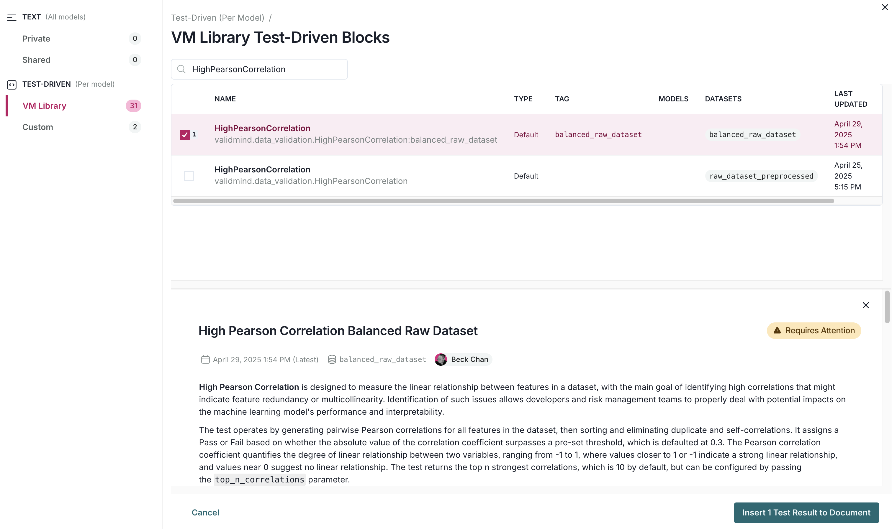
    • Click on VM Library under TEST-DRIVEN in the left sidebar.
    • In the search bar, type in HighPearsonCorrelation.
    • Select HighPearsonCorrelation:balanced_raw_dataset as the test.

    A preview of the test gets shown:

    Screenshot showing the HighPearsonCorrelation test selected

  6. Finally, click Insert 1 Test Result to Document to add the test result to the documentation.

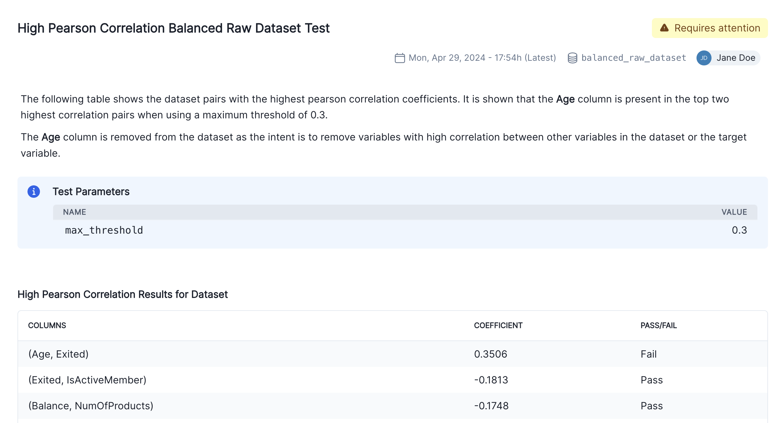
    Confirm that the individual results for the high correlation test has been correctly inserted into section 2.3. Correlations and Interactions of the documentation.

  7. Finalize the documentation by editing the test result's description block to explain the changes you made to the raw data and the reasons behind them as shown in the screenshot below:

    Screenshot showing the inserted High Pearson Correlation block

Running model evaluation tests

So far, we've focused on the data assessment and pre-processing that usually occurs prior to any models being built. Now, let's instead assume we have already built a model and we want to incorporate some model results into our documentation.

Train simple logistic regression model

Using ValidMind tests, we'll train a simple logistic regression model on our dataset and evaluate its performance by using the LogisticRegression class from the sklearn.linear_model.

To start, let's grab the first few rows from the balanced_raw_no_age_df dataset with the highly correlated features removed we initialized earlier:

balanced_raw_no_age_df.head()
CreditScore Geography Gender Tenure Balance NumOfProducts HasCrCard IsActiveMember EstimatedSalary Exited
290 640 France Male 9 0.00 2 1 1 199493.38 0
3374 705 France Male 3 0.00 2 0 0 129576.99 0
4805 684 France Male 0 0.00 2 1 1 36376.97 0
6545 659 France Female 3 0.00 1 1 0 183399.12 1
2752 713 France Male 6 94598.48 1 0 0 197519.66 1

Before training the model, we need to encode the categorical features in the dataset:

  • Use the OneHotEncoder class from the sklearn.preprocessing module to encode the categorical features.
  • The categorical features in the dataset are Geography and Gender.
balanced_raw_no_age_df = pd.get_dummies(
    balanced_raw_no_age_df, columns=["Geography", "Gender"], drop_first=True
)
balanced_raw_no_age_df.head()
CreditScore Tenure Balance NumOfProducts HasCrCard IsActiveMember EstimatedSalary Exited Geography_Germany Geography_Spain Gender_Male
290 640 9 0.00 2 1 1 199493.38 0 False False True
3374 705 3 0.00 2 0 0 129576.99 0 False False True
4805 684 0 0.00 2 1 1 36376.97 0 False False True
6545 659 3 0.00 1 1 0 183399.12 1 False False False
2752 713 6 94598.48 1 0 0 197519.66 1 False False True

We'll split our preprocessed dataset into training and testing, to help assess how well the model generalizes to unseen data:

  • We start by dividing our balanced_raw_no_age_df dataset into training and test subsets using train_test_split, with 80% of the data allocated to training (train_df) and 20% to testing (test_df).
  • From each subset, we separate the features (all columns except "Exited") into X_train and X_test, and the target column ("Exited") into y_train and y_test.
from sklearn.model_selection import train_test_split

train_df, test_df = train_test_split(balanced_raw_no_age_df, test_size=0.20)

X_train = train_df.drop("Exited", axis=1)
y_train = train_df["Exited"]
X_test = test_df.drop("Exited", axis=1)
y_test = test_df["Exited"]

Then using GridSearchCV, we'll find the best-performing hyperparameters or settings and save them:

from sklearn.linear_model import LogisticRegression

# Logistic Regression grid params
log_reg_params = {
    "penalty": ["l1", "l2"],
    "C": [0.001, 0.01, 0.1, 1, 10, 100, 1000],
    "solver": ["liblinear"],
}

# Grid search for Logistic Regression
from sklearn.model_selection import GridSearchCV

grid_log_reg = GridSearchCV(LogisticRegression(), log_reg_params)
grid_log_reg.fit(X_train, y_train)

# Logistic Regression best estimator
log_reg = grid_log_reg.best_estimator_
/opt/hostedtoolcache/Python/3.11.15/x64/lib/python3.11/site-packages/sklearn/linear_model/_logistic.py:1403: FutureWarning: 'penalty' was deprecated in version 1.8 and will be removed in 1.10. To avoid this warning, leave 'penalty' set to its default value and use 'l1_ratio' or 'C' instead. Use l1_ratio=0 instead of penalty='l2', l1_ratio=1 instead of penalty='l1', l1_ratio set to a float between 0 and 1 instead of penalty='elasticnet', and C=np.inf instead of penalty=None.
  warnings.warn(
/opt/hostedtoolcache/Python/3.11.15/x64/lib/python3.11/site-packages/sklearn/linear_model/_logistic.py:1429: UserWarning: Inconsistent values: penalty=l1 with l1_ratio=0.0. penalty is deprecated. Please use l1_ratio only.
  warnings.warn(
/opt/hostedtoolcache/Python/3.11.15/x64/lib/python3.11/site-packages/sklearn/linear_model/_logistic.py:1403: FutureWarning: 'penalty' was deprecated in version 1.8 and will be removed in 1.10. To avoid this warning, leave 'penalty' set to its default value and use 'l1_ratio' or 'C' instead. Use l1_ratio=0 instead of penalty='l2', l1_ratio=1 instead of penalty='l1', l1_ratio set to a float between 0 and 1 instead of penalty='elasticnet', and C=np.inf instead of penalty=None.
  warnings.warn(
/opt/hostedtoolcache/Python/3.11.15/x64/lib/python3.11/site-packages/sklearn/linear_model/_logistic.py:1429: UserWarning: Inconsistent values: penalty=l1 with l1_ratio=0.0. penalty is deprecated. Please use l1_ratio only.
  warnings.warn(
/opt/hostedtoolcache/Python/3.11.15/x64/lib/python3.11/site-packages/sklearn/linear_model/_logistic.py:1403: FutureWarning: 'penalty' was deprecated in version 1.8 and will be removed in 1.10. To avoid this warning, leave 'penalty' set to its default value and use 'l1_ratio' or 'C' instead. Use l1_ratio=0 instead of penalty='l2', l1_ratio=1 instead of penalty='l1', l1_ratio set to a float between 0 and 1 instead of penalty='elasticnet', and C=np.inf instead of penalty=None.
  warnings.warn(
/opt/hostedtoolcache/Python/3.11.15/x64/lib/python3.11/site-packages/sklearn/linear_model/_logistic.py:1429: UserWarning: Inconsistent values: penalty=l1 with l1_ratio=0.0. penalty is deprecated. Please use l1_ratio only.
  warnings.warn(
/opt/hostedtoolcache/Python/3.11.15/x64/lib/python3.11/site-packages/sklearn/linear_model/_logistic.py:1403: FutureWarning: 'penalty' was deprecated in version 1.8 and will be removed in 1.10. To avoid this warning, leave 'penalty' set to its default value and use 'l1_ratio' or 'C' instead. Use l1_ratio=0 instead of penalty='l2', l1_ratio=1 instead of penalty='l1', l1_ratio set to a float between 0 and 1 instead of penalty='elasticnet', and C=np.inf instead of penalty=None.
  warnings.warn(
/opt/hostedtoolcache/Python/3.11.15/x64/lib/python3.11/site-packages/sklearn/linear_model/_logistic.py:1429: UserWarning: Inconsistent values: penalty=l1 with l1_ratio=0.0. penalty is deprecated. Please use l1_ratio only.
  warnings.warn(
/opt/hostedtoolcache/Python/3.11.15/x64/lib/python3.11/site-packages/sklearn/linear_model/_logistic.py:1403: FutureWarning: 'penalty' was deprecated in version 1.8 and will be removed in 1.10. To avoid this warning, leave 'penalty' set to its default value and use 'l1_ratio' or 'C' instead. Use l1_ratio=0 instead of penalty='l2', l1_ratio=1 instead of penalty='l1', l1_ratio set to a float between 0 and 1 instead of penalty='elasticnet', and C=np.inf instead of penalty=None.
  warnings.warn(
/opt/hostedtoolcache/Python/3.11.15/x64/lib/python3.11/site-packages/sklearn/linear_model/_logistic.py:1429: UserWarning: Inconsistent values: penalty=l1 with l1_ratio=0.0. penalty is deprecated. Please use l1_ratio only.
  warnings.warn(
/opt/hostedtoolcache/Python/3.11.15/x64/lib/python3.11/site-packages/sklearn/linear_model/_logistic.py:1403: FutureWarning: 'penalty' was deprecated in version 1.8 and will be removed in 1.10. To avoid this warning, leave 'penalty' set to its default value and use 'l1_ratio' or 'C' instead. Use l1_ratio=0 instead of penalty='l2', l1_ratio=1 instead of penalty='l1', l1_ratio set to a float between 0 and 1 instead of penalty='elasticnet', and C=np.inf instead of penalty=None.
  warnings.warn(
/opt/hostedtoolcache/Python/3.11.15/x64/lib/python3.11/site-packages/sklearn/linear_model/_logistic.py:1403: FutureWarning: 'penalty' was deprecated in version 1.8 and will be removed in 1.10. To avoid this warning, leave 'penalty' set to its default value and use 'l1_ratio' or 'C' instead. Use l1_ratio=0 instead of penalty='l2', l1_ratio=1 instead of penalty='l1', l1_ratio set to a float between 0 and 1 instead of penalty='elasticnet', and C=np.inf instead of penalty=None.
  warnings.warn(
/opt/hostedtoolcache/Python/3.11.15/x64/lib/python3.11/site-packages/sklearn/linear_model/_logistic.py:1403: FutureWarning: 'penalty' was deprecated in version 1.8 and will be removed in 1.10. To avoid this warning, leave 'penalty' set to its default value and use 'l1_ratio' or 'C' instead. Use l1_ratio=0 instead of penalty='l2', l1_ratio=1 instead of penalty='l1', l1_ratio set to a float between 0 and 1 instead of penalty='elasticnet', and C=np.inf instead of penalty=None.
  warnings.warn(
/opt/hostedtoolcache/Python/3.11.15/x64/lib/python3.11/site-packages/sklearn/linear_model/_logistic.py:1403: FutureWarning: 'penalty' was deprecated in version 1.8 and will be removed in 1.10. To avoid this warning, leave 'penalty' set to its default value and use 'l1_ratio' or 'C' instead. Use l1_ratio=0 instead of penalty='l2', l1_ratio=1 instead of penalty='l1', l1_ratio set to a float between 0 and 1 instead of penalty='elasticnet', and C=np.inf instead of penalty=None.
  warnings.warn(
/opt/hostedtoolcache/Python/3.11.15/x64/lib/python3.11/site-packages/sklearn/linear_model/_logistic.py:1403: FutureWarning: 'penalty' was deprecated in version 1.8 and will be removed in 1.10. To avoid this warning, leave 'penalty' set to its default value and use 'l1_ratio' or 'C' instead. Use l1_ratio=0 instead of penalty='l2', l1_ratio=1 instead of penalty='l1', l1_ratio set to a float between 0 and 1 instead of penalty='elasticnet', and C=np.inf instead of penalty=None.
  warnings.warn(
/opt/hostedtoolcache/Python/3.11.15/x64/lib/python3.11/site-packages/sklearn/linear_model/_logistic.py:1403: FutureWarning: 'penalty' was deprecated in version 1.8 and will be removed in 1.10. To avoid this warning, leave 'penalty' set to its default value and use 'l1_ratio' or 'C' instead. Use l1_ratio=0 instead of penalty='l2', l1_ratio=1 instead of penalty='l1', l1_ratio set to a float between 0 and 1 instead of penalty='elasticnet', and C=np.inf instead of penalty=None.
  warnings.warn(
/opt/hostedtoolcache/Python/3.11.15/x64/lib/python3.11/site-packages/sklearn/linear_model/_logistic.py:1429: UserWarning: Inconsistent values: penalty=l1 with l1_ratio=0.0. penalty is deprecated. Please use l1_ratio only.
  warnings.warn(
/opt/hostedtoolcache/Python/3.11.15/x64/lib/python3.11/site-packages/sklearn/linear_model/_logistic.py:1403: FutureWarning: 'penalty' was deprecated in version 1.8 and will be removed in 1.10. To avoid this warning, leave 'penalty' set to its default value and use 'l1_ratio' or 'C' instead. Use l1_ratio=0 instead of penalty='l2', l1_ratio=1 instead of penalty='l1', l1_ratio set to a float between 0 and 1 instead of penalty='elasticnet', and C=np.inf instead of penalty=None.
  warnings.warn(
/opt/hostedtoolcache/Python/3.11.15/x64/lib/python3.11/site-packages/sklearn/linear_model/_logistic.py:1429: UserWarning: Inconsistent values: penalty=l1 with l1_ratio=0.0. penalty is deprecated. Please use l1_ratio only.
  warnings.warn(
/opt/hostedtoolcache/Python/3.11.15/x64/lib/python3.11/site-packages/sklearn/linear_model/_logistic.py:1403: FutureWarning: 'penalty' was deprecated in version 1.8 and will be removed in 1.10. To avoid this warning, leave 'penalty' set to its default value and use 'l1_ratio' or 'C' instead. Use l1_ratio=0 instead of penalty='l2', l1_ratio=1 instead of penalty='l1', l1_ratio set to a float between 0 and 1 instead of penalty='elasticnet', and C=np.inf instead of penalty=None.
  warnings.warn(
/opt/hostedtoolcache/Python/3.11.15/x64/lib/python3.11/site-packages/sklearn/linear_model/_logistic.py:1429: UserWarning: Inconsistent values: penalty=l1 with l1_ratio=0.0. penalty is deprecated. Please use l1_ratio only.
  warnings.warn(
/opt/hostedtoolcache/Python/3.11.15/x64/lib/python3.11/site-packages/sklearn/linear_model/_logistic.py:1403: FutureWarning: 'penalty' was deprecated in version 1.8 and will be removed in 1.10. To avoid this warning, leave 'penalty' set to its default value and use 'l1_ratio' or 'C' instead. Use l1_ratio=0 instead of penalty='l2', l1_ratio=1 instead of penalty='l1', l1_ratio set to a float between 0 and 1 instead of penalty='elasticnet', and C=np.inf instead of penalty=None.
  warnings.warn(
/opt/hostedtoolcache/Python/3.11.15/x64/lib/python3.11/site-packages/sklearn/linear_model/_logistic.py:1429: UserWarning: Inconsistent values: penalty=l1 with l1_ratio=0.0. penalty is deprecated. Please use l1_ratio only.
  warnings.warn(
/opt/hostedtoolcache/Python/3.11.15/x64/lib/python3.11/site-packages/sklearn/linear_model/_logistic.py:1403: FutureWarning: 'penalty' was deprecated in version 1.8 and will be removed in 1.10. To avoid this warning, leave 'penalty' set to its default value and use 'l1_ratio' or 'C' instead. Use l1_ratio=0 instead of penalty='l2', l1_ratio=1 instead of penalty='l1', l1_ratio set to a float between 0 and 1 instead of penalty='elasticnet', and C=np.inf instead of penalty=None.
  warnings.warn(
/opt/hostedtoolcache/Python/3.11.15/x64/lib/python3.11/site-packages/sklearn/linear_model/_logistic.py:1429: UserWarning: Inconsistent values: penalty=l1 with l1_ratio=0.0. penalty is deprecated. Please use l1_ratio only.
  warnings.warn(
/opt/hostedtoolcache/Python/3.11.15/x64/lib/python3.11/site-packages/sklearn/linear_model/_logistic.py:1403: FutureWarning: 'penalty' was deprecated in version 1.8 and will be removed in 1.10. To avoid this warning, leave 'penalty' set to its default value and use 'l1_ratio' or 'C' instead. Use l1_ratio=0 instead of penalty='l2', l1_ratio=1 instead of penalty='l1', l1_ratio set to a float between 0 and 1 instead of penalty='elasticnet', and C=np.inf instead of penalty=None.
  warnings.warn(
/opt/hostedtoolcache/Python/3.11.15/x64/lib/python3.11/site-packages/sklearn/linear_model/_logistic.py:1403: FutureWarning: 'penalty' was deprecated in version 1.8 and will be removed in 1.10. To avoid this warning, leave 'penalty' set to its default value and use 'l1_ratio' or 'C' instead. Use l1_ratio=0 instead of penalty='l2', l1_ratio=1 instead of penalty='l1', l1_ratio set to a float between 0 and 1 instead of penalty='elasticnet', and C=np.inf instead of penalty=None.
  warnings.warn(
/opt/hostedtoolcache/Python/3.11.15/x64/lib/python3.11/site-packages/sklearn/linear_model/_logistic.py:1403: FutureWarning: 'penalty' was deprecated in version 1.8 and will be removed in 1.10. To avoid this warning, leave 'penalty' set to its default value and use 'l1_ratio' or 'C' instead. Use l1_ratio=0 instead of penalty='l2', l1_ratio=1 instead of penalty='l1', l1_ratio set to a float between 0 and 1 instead of penalty='elasticnet', and C=np.inf instead of penalty=None.
  warnings.warn(
/opt/hostedtoolcache/Python/3.11.15/x64/lib/python3.11/site-packages/sklearn/linear_model/_logistic.py:1403: FutureWarning: 'penalty' was deprecated in version 1.8 and will be removed in 1.10. To avoid this warning, leave 'penalty' set to its default value and use 'l1_ratio' or 'C' instead. Use l1_ratio=0 instead of penalty='l2', l1_ratio=1 instead of penalty='l1', l1_ratio set to a float between 0 and 1 instead of penalty='elasticnet', and C=np.inf instead of penalty=None.
  warnings.warn(
/opt/hostedtoolcache/Python/3.11.15/x64/lib/python3.11/site-packages/sklearn/linear_model/_logistic.py:1403: FutureWarning: 'penalty' was deprecated in version 1.8 and will be removed in 1.10. To avoid this warning, leave 'penalty' set to its default value and use 'l1_ratio' or 'C' instead. Use l1_ratio=0 instead of penalty='l2', l1_ratio=1 instead of penalty='l1', l1_ratio set to a float between 0 and 1 instead of penalty='elasticnet', and C=np.inf instead of penalty=None.
  warnings.warn(
/opt/hostedtoolcache/Python/3.11.15/x64/lib/python3.11/site-packages/sklearn/linear_model/_logistic.py:1403: FutureWarning: 'penalty' was deprecated in version 1.8 and will be removed in 1.10. To avoid this warning, leave 'penalty' set to its default value and use 'l1_ratio' or 'C' instead. Use l1_ratio=0 instead of penalty='l2', l1_ratio=1 instead of penalty='l1', l1_ratio set to a float between 0 and 1 instead of penalty='elasticnet', and C=np.inf instead of penalty=None.
  warnings.warn(
/opt/hostedtoolcache/Python/3.11.15/x64/lib/python3.11/site-packages/sklearn/linear_model/_logistic.py:1429: UserWarning: Inconsistent values: penalty=l1 with l1_ratio=0.0. penalty is deprecated. Please use l1_ratio only.
  warnings.warn(
/opt/hostedtoolcache/Python/3.11.15/x64/lib/python3.11/site-packages/sklearn/linear_model/_logistic.py:1403: FutureWarning: 'penalty' was deprecated in version 1.8 and will be removed in 1.10. To avoid this warning, leave 'penalty' set to its default value and use 'l1_ratio' or 'C' instead. Use l1_ratio=0 instead of penalty='l2', l1_ratio=1 instead of penalty='l1', l1_ratio set to a float between 0 and 1 instead of penalty='elasticnet', and C=np.inf instead of penalty=None.
  warnings.warn(
/opt/hostedtoolcache/Python/3.11.15/x64/lib/python3.11/site-packages/sklearn/linear_model/_logistic.py:1429: UserWarning: Inconsistent values: penalty=l1 with l1_ratio=0.0. penalty is deprecated. Please use l1_ratio only.
  warnings.warn(
/opt/hostedtoolcache/Python/3.11.15/x64/lib/python3.11/site-packages/sklearn/linear_model/_logistic.py:1403: FutureWarning: 'penalty' was deprecated in version 1.8 and will be removed in 1.10. To avoid this warning, leave 'penalty' set to its default value and use 'l1_ratio' or 'C' instead. Use l1_ratio=0 instead of penalty='l2', l1_ratio=1 instead of penalty='l1', l1_ratio set to a float between 0 and 1 instead of penalty='elasticnet', and C=np.inf instead of penalty=None.
  warnings.warn(
/opt/hostedtoolcache/Python/3.11.15/x64/lib/python3.11/site-packages/sklearn/linear_model/_logistic.py:1429: UserWarning: Inconsistent values: penalty=l1 with l1_ratio=0.0. penalty is deprecated. Please use l1_ratio only.
  warnings.warn(
/opt/hostedtoolcache/Python/3.11.15/x64/lib/python3.11/site-packages/sklearn/linear_model/_logistic.py:1403: FutureWarning: 'penalty' was deprecated in version 1.8 and will be removed in 1.10. To avoid this warning, leave 'penalty' set to its default value and use 'l1_ratio' or 'C' instead. Use l1_ratio=0 instead of penalty='l2', l1_ratio=1 instead of penalty='l1', l1_ratio set to a float between 0 and 1 instead of penalty='elasticnet', and C=np.inf instead of penalty=None.
  warnings.warn(
/opt/hostedtoolcache/Python/3.11.15/x64/lib/python3.11/site-packages/sklearn/linear_model/_logistic.py:1429: UserWarning: Inconsistent values: penalty=l1 with l1_ratio=0.0. penalty is deprecated. Please use l1_ratio only.
  warnings.warn(
/opt/hostedtoolcache/Python/3.11.15/x64/lib/python3.11/site-packages/sklearn/linear_model/_logistic.py:1403: FutureWarning: 'penalty' was deprecated in version 1.8 and will be removed in 1.10. To avoid this warning, leave 'penalty' set to its default value and use 'l1_ratio' or 'C' instead. Use l1_ratio=0 instead of penalty='l2', l1_ratio=1 instead of penalty='l1', l1_ratio set to a float between 0 and 1 instead of penalty='elasticnet', and C=np.inf instead of penalty=None.
  warnings.warn(
/opt/hostedtoolcache/Python/3.11.15/x64/lib/python3.11/site-packages/sklearn/linear_model/_logistic.py:1429: UserWarning: Inconsistent values: penalty=l1 with l1_ratio=0.0. penalty is deprecated. Please use l1_ratio only.
  warnings.warn(
/opt/hostedtoolcache/Python/3.11.15/x64/lib/python3.11/site-packages/sklearn/linear_model/_logistic.py:1403: FutureWarning: 'penalty' was deprecated in version 1.8 and will be removed in 1.10. To avoid this warning, leave 'penalty' set to its default value and use 'l1_ratio' or 'C' instead. Use l1_ratio=0 instead of penalty='l2', l1_ratio=1 instead of penalty='l1', l1_ratio set to a float between 0 and 1 instead of penalty='elasticnet', and C=np.inf instead of penalty=None.
  warnings.warn(
/opt/hostedtoolcache/Python/3.11.15/x64/lib/python3.11/site-packages/sklearn/linear_model/_logistic.py:1403: FutureWarning: 'penalty' was deprecated in version 1.8 and will be removed in 1.10. To avoid this warning, leave 'penalty' set to its default value and use 'l1_ratio' or 'C' instead. Use l1_ratio=0 instead of penalty='l2', l1_ratio=1 instead of penalty='l1', l1_ratio set to a float between 0 and 1 instead of penalty='elasticnet', and C=np.inf instead of penalty=None.
  warnings.warn(
/opt/hostedtoolcache/Python/3.11.15/x64/lib/python3.11/site-packages/sklearn/linear_model/_logistic.py:1403: FutureWarning: 'penalty' was deprecated in version 1.8 and will be removed in 1.10. To avoid this warning, leave 'penalty' set to its default value and use 'l1_ratio' or 'C' instead. Use l1_ratio=0 instead of penalty='l2', l1_ratio=1 instead of penalty='l1', l1_ratio set to a float between 0 and 1 instead of penalty='elasticnet', and C=np.inf instead of penalty=None.
  warnings.warn(
/opt/hostedtoolcache/Python/3.11.15/x64/lib/python3.11/site-packages/sklearn/linear_model/_logistic.py:1403: FutureWarning: 'penalty' was deprecated in version 1.8 and will be removed in 1.10. To avoid this warning, leave 'penalty' set to its default value and use 'l1_ratio' or 'C' instead. Use l1_ratio=0 instead of penalty='l2', l1_ratio=1 instead of penalty='l1', l1_ratio set to a float between 0 and 1 instead of penalty='elasticnet', and C=np.inf instead of penalty=None.
  warnings.warn(
/opt/hostedtoolcache/Python/3.11.15/x64/lib/python3.11/site-packages/sklearn/linear_model/_logistic.py:1403: FutureWarning: 'penalty' was deprecated in version 1.8 and will be removed in 1.10. To avoid this warning, leave 'penalty' set to its default value and use 'l1_ratio' or 'C' instead. Use l1_ratio=0 instead of penalty='l2', l1_ratio=1 instead of penalty='l1', l1_ratio set to a float between 0 and 1 instead of penalty='elasticnet', and C=np.inf instead of penalty=None.
  warnings.warn(
/opt/hostedtoolcache/Python/3.11.15/x64/lib/python3.11/site-packages/sklearn/linear_model/_logistic.py:1403: FutureWarning: 'penalty' was deprecated in version 1.8 and will be removed in 1.10. To avoid this warning, leave 'penalty' set to its default value and use 'l1_ratio' or 'C' instead. Use l1_ratio=0 instead of penalty='l2', l1_ratio=1 instead of penalty='l1', l1_ratio set to a float between 0 and 1 instead of penalty='elasticnet', and C=np.inf instead of penalty=None.
  warnings.warn(
/opt/hostedtoolcache/Python/3.11.15/x64/lib/python3.11/site-packages/sklearn/linear_model/_logistic.py:1429: UserWarning: Inconsistent values: penalty=l1 with l1_ratio=0.0. penalty is deprecated. Please use l1_ratio only.
  warnings.warn(
/opt/hostedtoolcache/Python/3.11.15/x64/lib/python3.11/site-packages/sklearn/linear_model/_logistic.py:1403: FutureWarning: 'penalty' was deprecated in version 1.8 and will be removed in 1.10. To avoid this warning, leave 'penalty' set to its default value and use 'l1_ratio' or 'C' instead. Use l1_ratio=0 instead of penalty='l2', l1_ratio=1 instead of penalty='l1', l1_ratio set to a float between 0 and 1 instead of penalty='elasticnet', and C=np.inf instead of penalty=None.
  warnings.warn(
/opt/hostedtoolcache/Python/3.11.15/x64/lib/python3.11/site-packages/sklearn/linear_model/_logistic.py:1429: UserWarning: Inconsistent values: penalty=l1 with l1_ratio=0.0. penalty is deprecated. Please use l1_ratio only.
  warnings.warn(
/opt/hostedtoolcache/Python/3.11.15/x64/lib/python3.11/site-packages/sklearn/linear_model/_logistic.py:1403: FutureWarning: 'penalty' was deprecated in version 1.8 and will be removed in 1.10. To avoid this warning, leave 'penalty' set to its default value and use 'l1_ratio' or 'C' instead. Use l1_ratio=0 instead of penalty='l2', l1_ratio=1 instead of penalty='l1', l1_ratio set to a float between 0 and 1 instead of penalty='elasticnet', and C=np.inf instead of penalty=None.
  warnings.warn(
/opt/hostedtoolcache/Python/3.11.15/x64/lib/python3.11/site-packages/sklearn/linear_model/_logistic.py:1429: UserWarning: Inconsistent values: penalty=l1 with l1_ratio=0.0. penalty is deprecated. Please use l1_ratio only.
  warnings.warn(
/opt/hostedtoolcache/Python/3.11.15/x64/lib/python3.11/site-packages/sklearn/linear_model/_logistic.py:1403: FutureWarning: 'penalty' was deprecated in version 1.8 and will be removed in 1.10. To avoid this warning, leave 'penalty' set to its default value and use 'l1_ratio' or 'C' instead. Use l1_ratio=0 instead of penalty='l2', l1_ratio=1 instead of penalty='l1', l1_ratio set to a float between 0 and 1 instead of penalty='elasticnet', and C=np.inf instead of penalty=None.
  warnings.warn(
/opt/hostedtoolcache/Python/3.11.15/x64/lib/python3.11/site-packages/sklearn/linear_model/_logistic.py:1429: UserWarning: Inconsistent values: penalty=l1 with l1_ratio=0.0. penalty is deprecated. Please use l1_ratio only.
  warnings.warn(
/opt/hostedtoolcache/Python/3.11.15/x64/lib/python3.11/site-packages/sklearn/linear_model/_logistic.py:1403: FutureWarning: 'penalty' was deprecated in version 1.8 and will be removed in 1.10. To avoid this warning, leave 'penalty' set to its default value and use 'l1_ratio' or 'C' instead. Use l1_ratio=0 instead of penalty='l2', l1_ratio=1 instead of penalty='l1', l1_ratio set to a float between 0 and 1 instead of penalty='elasticnet', and C=np.inf instead of penalty=None.
  warnings.warn(
/opt/hostedtoolcache/Python/3.11.15/x64/lib/python3.11/site-packages/sklearn/linear_model/_logistic.py:1429: UserWarning: Inconsistent values: penalty=l1 with l1_ratio=0.0. penalty is deprecated. Please use l1_ratio only.
  warnings.warn(
/opt/hostedtoolcache/Python/3.11.15/x64/lib/python3.11/site-packages/sklearn/linear_model/_logistic.py:1403: FutureWarning: 'penalty' was deprecated in version 1.8 and will be removed in 1.10. To avoid this warning, leave 'penalty' set to its default value and use 'l1_ratio' or 'C' instead. Use l1_ratio=0 instead of penalty='l2', l1_ratio=1 instead of penalty='l1', l1_ratio set to a float between 0 and 1 instead of penalty='elasticnet', and C=np.inf instead of penalty=None.
  warnings.warn(
/opt/hostedtoolcache/Python/3.11.15/x64/lib/python3.11/site-packages/sklearn/linear_model/_logistic.py:1403: FutureWarning: 'penalty' was deprecated in version 1.8 and will be removed in 1.10. To avoid this warning, leave 'penalty' set to its default value and use 'l1_ratio' or 'C' instead. Use l1_ratio=0 instead of penalty='l2', l1_ratio=1 instead of penalty='l1', l1_ratio set to a float between 0 and 1 instead of penalty='elasticnet', and C=np.inf instead of penalty=None.
  warnings.warn(
/opt/hostedtoolcache/Python/3.11.15/x64/lib/python3.11/site-packages/sklearn/linear_model/_logistic.py:1403: FutureWarning: 'penalty' was deprecated in version 1.8 and will be removed in 1.10. To avoid this warning, leave 'penalty' set to its default value and use 'l1_ratio' or 'C' instead. Use l1_ratio=0 instead of penalty='l2', l1_ratio=1 instead of penalty='l1', l1_ratio set to a float between 0 and 1 instead of penalty='elasticnet', and C=np.inf instead of penalty=None.
  warnings.warn(
/opt/hostedtoolcache/Python/3.11.15/x64/lib/python3.11/site-packages/sklearn/linear_model/_logistic.py:1403: FutureWarning: 'penalty' was deprecated in version 1.8 and will be removed in 1.10. To avoid this warning, leave 'penalty' set to its default value and use 'l1_ratio' or 'C' instead. Use l1_ratio=0 instead of penalty='l2', l1_ratio=1 instead of penalty='l1', l1_ratio set to a float between 0 and 1 instead of penalty='elasticnet', and C=np.inf instead of penalty=None.
  warnings.warn(
/opt/hostedtoolcache/Python/3.11.15/x64/lib/python3.11/site-packages/sklearn/linear_model/_logistic.py:1403: FutureWarning: 'penalty' was deprecated in version 1.8 and will be removed in 1.10. To avoid this warning, leave 'penalty' set to its default value and use 'l1_ratio' or 'C' instead. Use l1_ratio=0 instead of penalty='l2', l1_ratio=1 instead of penalty='l1', l1_ratio set to a float between 0 and 1 instead of penalty='elasticnet', and C=np.inf instead of penalty=None.
  warnings.warn(
/opt/hostedtoolcache/Python/3.11.15/x64/lib/python3.11/site-packages/sklearn/linear_model/_logistic.py:1403: FutureWarning: 'penalty' was deprecated in version 1.8 and will be removed in 1.10. To avoid this warning, leave 'penalty' set to its default value and use 'l1_ratio' or 'C' instead. Use l1_ratio=0 instead of penalty='l2', l1_ratio=1 instead of penalty='l1', l1_ratio set to a float between 0 and 1 instead of penalty='elasticnet', and C=np.inf instead of penalty=None.
  warnings.warn(
/opt/hostedtoolcache/Python/3.11.15/x64/lib/python3.11/site-packages/sklearn/linear_model/_logistic.py:1429: UserWarning: Inconsistent values: penalty=l1 with l1_ratio=0.0. penalty is deprecated. Please use l1_ratio only.
  warnings.warn(
/opt/hostedtoolcache/Python/3.11.15/x64/lib/python3.11/site-packages/sklearn/linear_model/_logistic.py:1403: FutureWarning: 'penalty' was deprecated in version 1.8 and will be removed in 1.10. To avoid this warning, leave 'penalty' set to its default value and use 'l1_ratio' or 'C' instead. Use l1_ratio=0 instead of penalty='l2', l1_ratio=1 instead of penalty='l1', l1_ratio set to a float between 0 and 1 instead of penalty='elasticnet', and C=np.inf instead of penalty=None.
  warnings.warn(
/opt/hostedtoolcache/Python/3.11.15/x64/lib/python3.11/site-packages/sklearn/linear_model/_logistic.py:1429: UserWarning: Inconsistent values: penalty=l1 with l1_ratio=0.0. penalty is deprecated. Please use l1_ratio only.
  warnings.warn(
/opt/hostedtoolcache/Python/3.11.15/x64/lib/python3.11/site-packages/sklearn/linear_model/_logistic.py:1403: FutureWarning: 'penalty' was deprecated in version 1.8 and will be removed in 1.10. To avoid this warning, leave 'penalty' set to its default value and use 'l1_ratio' or 'C' instead. Use l1_ratio=0 instead of penalty='l2', l1_ratio=1 instead of penalty='l1', l1_ratio set to a float between 0 and 1 instead of penalty='elasticnet', and C=np.inf instead of penalty=None.
  warnings.warn(
/opt/hostedtoolcache/Python/3.11.15/x64/lib/python3.11/site-packages/sklearn/linear_model/_logistic.py:1429: UserWarning: Inconsistent values: penalty=l1 with l1_ratio=0.0. penalty is deprecated. Please use l1_ratio only.
  warnings.warn(
/opt/hostedtoolcache/Python/3.11.15/x64/lib/python3.11/site-packages/sklearn/linear_model/_logistic.py:1403: FutureWarning: 'penalty' was deprecated in version 1.8 and will be removed in 1.10. To avoid this warning, leave 'penalty' set to its default value and use 'l1_ratio' or 'C' instead. Use l1_ratio=0 instead of penalty='l2', l1_ratio=1 instead of penalty='l1', l1_ratio set to a float between 0 and 1 instead of penalty='elasticnet', and C=np.inf instead of penalty=None.
  warnings.warn(
/opt/hostedtoolcache/Python/3.11.15/x64/lib/python3.11/site-packages/sklearn/linear_model/_logistic.py:1429: UserWarning: Inconsistent values: penalty=l1 with l1_ratio=0.0. penalty is deprecated. Please use l1_ratio only.
  warnings.warn(
/opt/hostedtoolcache/Python/3.11.15/x64/lib/python3.11/site-packages/sklearn/linear_model/_logistic.py:1403: FutureWarning: 'penalty' was deprecated in version 1.8 and will be removed in 1.10. To avoid this warning, leave 'penalty' set to its default value and use 'l1_ratio' or 'C' instead. Use l1_ratio=0 instead of penalty='l2', l1_ratio=1 instead of penalty='l1', l1_ratio set to a float between 0 and 1 instead of penalty='elasticnet', and C=np.inf instead of penalty=None.
  warnings.warn(
/opt/hostedtoolcache/Python/3.11.15/x64/lib/python3.11/site-packages/sklearn/linear_model/_logistic.py:1429: UserWarning: Inconsistent values: penalty=l1 with l1_ratio=0.0. penalty is deprecated. Please use l1_ratio only.
  warnings.warn(
/opt/hostedtoolcache/Python/3.11.15/x64/lib/python3.11/site-packages/sklearn/linear_model/_logistic.py:1403: FutureWarning: 'penalty' was deprecated in version 1.8 and will be removed in 1.10. To avoid this warning, leave 'penalty' set to its default value and use 'l1_ratio' or 'C' instead. Use l1_ratio=0 instead of penalty='l2', l1_ratio=1 instead of penalty='l1', l1_ratio set to a float between 0 and 1 instead of penalty='elasticnet', and C=np.inf instead of penalty=None.
  warnings.warn(
/opt/hostedtoolcache/Python/3.11.15/x64/lib/python3.11/site-packages/sklearn/linear_model/_logistic.py:1403: FutureWarning: 'penalty' was deprecated in version 1.8 and will be removed in 1.10. To avoid this warning, leave 'penalty' set to its default value and use 'l1_ratio' or 'C' instead. Use l1_ratio=0 instead of penalty='l2', l1_ratio=1 instead of penalty='l1', l1_ratio set to a float between 0 and 1 instead of penalty='elasticnet', and C=np.inf instead of penalty=None.
  warnings.warn(
/opt/hostedtoolcache/Python/3.11.15/x64/lib/python3.11/site-packages/sklearn/linear_model/_logistic.py:1403: FutureWarning: 'penalty' was deprecated in version 1.8 and will be removed in 1.10. To avoid this warning, leave 'penalty' set to its default value and use 'l1_ratio' or 'C' instead. Use l1_ratio=0 instead of penalty='l2', l1_ratio=1 instead of penalty='l1', l1_ratio set to a float between 0 and 1 instead of penalty='elasticnet', and C=np.inf instead of penalty=None.
  warnings.warn(
/opt/hostedtoolcache/Python/3.11.15/x64/lib/python3.11/site-packages/sklearn/linear_model/_logistic.py:1403: FutureWarning: 'penalty' was deprecated in version 1.8 and will be removed in 1.10. To avoid this warning, leave 'penalty' set to its default value and use 'l1_ratio' or 'C' instead. Use l1_ratio=0 instead of penalty='l2', l1_ratio=1 instead of penalty='l1', l1_ratio set to a float between 0 and 1 instead of penalty='elasticnet', and C=np.inf instead of penalty=None.
  warnings.warn(
/opt/hostedtoolcache/Python/3.11.15/x64/lib/python3.11/site-packages/sklearn/linear_model/_logistic.py:1403: FutureWarning: 'penalty' was deprecated in version 1.8 and will be removed in 1.10. To avoid this warning, leave 'penalty' set to its default value and use 'l1_ratio' or 'C' instead. Use l1_ratio=0 instead of penalty='l2', l1_ratio=1 instead of penalty='l1', l1_ratio set to a float between 0 and 1 instead of penalty='elasticnet', and C=np.inf instead of penalty=None.
  warnings.warn(
/opt/hostedtoolcache/Python/3.11.15/x64/lib/python3.11/site-packages/sklearn/linear_model/_logistic.py:1403: FutureWarning: 'penalty' was deprecated in version 1.8 and will be removed in 1.10. To avoid this warning, leave 'penalty' set to its default value and use 'l1_ratio' or 'C' instead. Use l1_ratio=0 instead of penalty='l2', l1_ratio=1 instead of penalty='l1', l1_ratio set to a float between 0 and 1 instead of penalty='elasticnet', and C=np.inf instead of penalty=None.
  warnings.warn(
/opt/hostedtoolcache/Python/3.11.15/x64/lib/python3.11/site-packages/sklearn/linear_model/_logistic.py:1429: UserWarning: Inconsistent values: penalty=l1 with l1_ratio=0.0. penalty is deprecated. Please use l1_ratio only.
  warnings.warn(
/opt/hostedtoolcache/Python/3.11.15/x64/lib/python3.11/site-packages/sklearn/linear_model/_logistic.py:1403: FutureWarning: 'penalty' was deprecated in version 1.8 and will be removed in 1.10. To avoid this warning, leave 'penalty' set to its default value and use 'l1_ratio' or 'C' instead. Use l1_ratio=0 instead of penalty='l2', l1_ratio=1 instead of penalty='l1', l1_ratio set to a float between 0 and 1 instead of penalty='elasticnet', and C=np.inf instead of penalty=None.
  warnings.warn(
/opt/hostedtoolcache/Python/3.11.15/x64/lib/python3.11/site-packages/sklearn/linear_model/_logistic.py:1429: UserWarning: Inconsistent values: penalty=l1 with l1_ratio=0.0. penalty is deprecated. Please use l1_ratio only.
  warnings.warn(
/opt/hostedtoolcache/Python/3.11.15/x64/lib/python3.11/site-packages/sklearn/linear_model/_logistic.py:1403: FutureWarning: 'penalty' was deprecated in version 1.8 and will be removed in 1.10. To avoid this warning, leave 'penalty' set to its default value and use 'l1_ratio' or 'C' instead. Use l1_ratio=0 instead of penalty='l2', l1_ratio=1 instead of penalty='l1', l1_ratio set to a float between 0 and 1 instead of penalty='elasticnet', and C=np.inf instead of penalty=None.
  warnings.warn(
/opt/hostedtoolcache/Python/3.11.15/x64/lib/python3.11/site-packages/sklearn/linear_model/_logistic.py:1429: UserWarning: Inconsistent values: penalty=l1 with l1_ratio=0.0. penalty is deprecated. Please use l1_ratio only.
  warnings.warn(
/opt/hostedtoolcache/Python/3.11.15/x64/lib/python3.11/site-packages/sklearn/linear_model/_logistic.py:1403: FutureWarning: 'penalty' was deprecated in version 1.8 and will be removed in 1.10. To avoid this warning, leave 'penalty' set to its default value and use 'l1_ratio' or 'C' instead. Use l1_ratio=0 instead of penalty='l2', l1_ratio=1 instead of penalty='l1', l1_ratio set to a float between 0 and 1 instead of penalty='elasticnet', and C=np.inf instead of penalty=None.
  warnings.warn(
/opt/hostedtoolcache/Python/3.11.15/x64/lib/python3.11/site-packages/sklearn/linear_model/_logistic.py:1429: UserWarning: Inconsistent values: penalty=l1 with l1_ratio=0.0. penalty is deprecated. Please use l1_ratio only.
  warnings.warn(
/opt/hostedtoolcache/Python/3.11.15/x64/lib/python3.11/site-packages/sklearn/linear_model/_logistic.py:1403: FutureWarning: 'penalty' was deprecated in version 1.8 and will be removed in 1.10. To avoid this warning, leave 'penalty' set to its default value and use 'l1_ratio' or 'C' instead. Use l1_ratio=0 instead of penalty='l2', l1_ratio=1 instead of penalty='l1', l1_ratio set to a float between 0 and 1 instead of penalty='elasticnet', and C=np.inf instead of penalty=None.
  warnings.warn(
/opt/hostedtoolcache/Python/3.11.15/x64/lib/python3.11/site-packages/sklearn/linear_model/_logistic.py:1429: UserWarning: Inconsistent values: penalty=l1 with l1_ratio=0.0. penalty is deprecated. Please use l1_ratio only.
  warnings.warn(
/opt/hostedtoolcache/Python/3.11.15/x64/lib/python3.11/site-packages/sklearn/linear_model/_logistic.py:1403: FutureWarning: 'penalty' was deprecated in version 1.8 and will be removed in 1.10. To avoid this warning, leave 'penalty' set to its default value and use 'l1_ratio' or 'C' instead. Use l1_ratio=0 instead of penalty='l2', l1_ratio=1 instead of penalty='l1', l1_ratio set to a float between 0 and 1 instead of penalty='elasticnet', and C=np.inf instead of penalty=None.
  warnings.warn(
/opt/hostedtoolcache/Python/3.11.15/x64/lib/python3.11/site-packages/sklearn/linear_model/_logistic.py:1403: FutureWarning: 'penalty' was deprecated in version 1.8 and will be removed in 1.10. To avoid this warning, leave 'penalty' set to its default value and use 'l1_ratio' or 'C' instead. Use l1_ratio=0 instead of penalty='l2', l1_ratio=1 instead of penalty='l1', l1_ratio set to a float between 0 and 1 instead of penalty='elasticnet', and C=np.inf instead of penalty=None.
  warnings.warn(
/opt/hostedtoolcache/Python/3.11.15/x64/lib/python3.11/site-packages/sklearn/linear_model/_logistic.py:1403: FutureWarning: 'penalty' was deprecated in version 1.8 and will be removed in 1.10. To avoid this warning, leave 'penalty' set to its default value and use 'l1_ratio' or 'C' instead. Use l1_ratio=0 instead of penalty='l2', l1_ratio=1 instead of penalty='l1', l1_ratio set to a float between 0 and 1 instead of penalty='elasticnet', and C=np.inf instead of penalty=None.
  warnings.warn(
/opt/hostedtoolcache/Python/3.11.15/x64/lib/python3.11/site-packages/sklearn/linear_model/_logistic.py:1403: FutureWarning: 'penalty' was deprecated in version 1.8 and will be removed in 1.10. To avoid this warning, leave 'penalty' set to its default value and use 'l1_ratio' or 'C' instead. Use l1_ratio=0 instead of penalty='l2', l1_ratio=1 instead of penalty='l1', l1_ratio set to a float between 0 and 1 instead of penalty='elasticnet', and C=np.inf instead of penalty=None.
  warnings.warn(
/opt/hostedtoolcache/Python/3.11.15/x64/lib/python3.11/site-packages/sklearn/linear_model/_logistic.py:1403: FutureWarning: 'penalty' was deprecated in version 1.8 and will be removed in 1.10. To avoid this warning, leave 'penalty' set to its default value and use 'l1_ratio' or 'C' instead. Use l1_ratio=0 instead of penalty='l2', l1_ratio=1 instead of penalty='l1', l1_ratio set to a float between 0 and 1 instead of penalty='elasticnet', and C=np.inf instead of penalty=None.
  warnings.warn(
/opt/hostedtoolcache/Python/3.11.15/x64/lib/python3.11/site-packages/sklearn/linear_model/_logistic.py:1403: FutureWarning: 'penalty' was deprecated in version 1.8 and will be removed in 1.10. To avoid this warning, leave 'penalty' set to its default value and use 'l1_ratio' or 'C' instead. Use l1_ratio=0 instead of penalty='l2', l1_ratio=1 instead of penalty='l1', l1_ratio set to a float between 0 and 1 instead of penalty='elasticnet', and C=np.inf instead of penalty=None.
  warnings.warn(
/opt/hostedtoolcache/Python/3.11.15/x64/lib/python3.11/site-packages/sklearn/linear_model/_logistic.py:1429: UserWarning: Inconsistent values: penalty=l1 with l1_ratio=0.0. penalty is deprecated. Please use l1_ratio only.
  warnings.warn(
/opt/hostedtoolcache/Python/3.11.15/x64/lib/python3.11/site-packages/sklearn/linear_model/_logistic.py:1403: FutureWarning: 'penalty' was deprecated in version 1.8 and will be removed in 1.10. To avoid this warning, leave 'penalty' set to its default value and use 'l1_ratio' or 'C' instead. Use l1_ratio=0 instead of penalty='l2', l1_ratio=1 instead of penalty='l1', l1_ratio set to a float between 0 and 1 instead of penalty='elasticnet', and C=np.inf instead of penalty=None.
  warnings.warn(
/opt/hostedtoolcache/Python/3.11.15/x64/lib/python3.11/site-packages/sklearn/linear_model/_logistic.py:1429: UserWarning: Inconsistent values: penalty=l1 with l1_ratio=0.0. penalty is deprecated. Please use l1_ratio only.
  warnings.warn(
/opt/hostedtoolcache/Python/3.11.15/x64/lib/python3.11/site-packages/sklearn/linear_model/_logistic.py:1403: FutureWarning: 'penalty' was deprecated in version 1.8 and will be removed in 1.10. To avoid this warning, leave 'penalty' set to its default value and use 'l1_ratio' or 'C' instead. Use l1_ratio=0 instead of penalty='l2', l1_ratio=1 instead of penalty='l1', l1_ratio set to a float between 0 and 1 instead of penalty='elasticnet', and C=np.inf instead of penalty=None.
  warnings.warn(
/opt/hostedtoolcache/Python/3.11.15/x64/lib/python3.11/site-packages/sklearn/linear_model/_logistic.py:1429: UserWarning: Inconsistent values: penalty=l1 with l1_ratio=0.0. penalty is deprecated. Please use l1_ratio only.
  warnings.warn(
/opt/hostedtoolcache/Python/3.11.15/x64/lib/python3.11/site-packages/sklearn/linear_model/_logistic.py:1403: FutureWarning: 'penalty' was deprecated in version 1.8 and will be removed in 1.10. To avoid this warning, leave 'penalty' set to its default value and use 'l1_ratio' or 'C' instead. Use l1_ratio=0 instead of penalty='l2', l1_ratio=1 instead of penalty='l1', l1_ratio set to a float between 0 and 1 instead of penalty='elasticnet', and C=np.inf instead of penalty=None.
  warnings.warn(
/opt/hostedtoolcache/Python/3.11.15/x64/lib/python3.11/site-packages/sklearn/linear_model/_logistic.py:1429: UserWarning: Inconsistent values: penalty=l1 with l1_ratio=0.0. penalty is deprecated. Please use l1_ratio only.
  warnings.warn(
/opt/hostedtoolcache/Python/3.11.15/x64/lib/python3.11/site-packages/sklearn/linear_model/_logistic.py:1403: FutureWarning: 'penalty' was deprecated in version 1.8 and will be removed in 1.10. To avoid this warning, leave 'penalty' set to its default value and use 'l1_ratio' or 'C' instead. Use l1_ratio=0 instead of penalty='l2', l1_ratio=1 instead of penalty='l1', l1_ratio set to a float between 0 and 1 instead of penalty='elasticnet', and C=np.inf instead of penalty=None.
  warnings.warn(
/opt/hostedtoolcache/Python/3.11.15/x64/lib/python3.11/site-packages/sklearn/linear_model/_logistic.py:1429: UserWarning: Inconsistent values: penalty=l1 with l1_ratio=0.0. penalty is deprecated. Please use l1_ratio only.
  warnings.warn(
/opt/hostedtoolcache/Python/3.11.15/x64/lib/python3.11/site-packages/sklearn/linear_model/_logistic.py:1403: FutureWarning: 'penalty' was deprecated in version 1.8 and will be removed in 1.10. To avoid this warning, leave 'penalty' set to its default value and use 'l1_ratio' or 'C' instead. Use l1_ratio=0 instead of penalty='l2', l1_ratio=1 instead of penalty='l1', l1_ratio set to a float between 0 and 1 instead of penalty='elasticnet', and C=np.inf instead of penalty=None.
  warnings.warn(
/opt/hostedtoolcache/Python/3.11.15/x64/lib/python3.11/site-packages/sklearn/linear_model/_logistic.py:1403: FutureWarning: 'penalty' was deprecated in version 1.8 and will be removed in 1.10. To avoid this warning, leave 'penalty' set to its default value and use 'l1_ratio' or 'C' instead. Use l1_ratio=0 instead of penalty='l2', l1_ratio=1 instead of penalty='l1', l1_ratio set to a float between 0 and 1 instead of penalty='elasticnet', and C=np.inf instead of penalty=None.
  warnings.warn(
/opt/hostedtoolcache/Python/3.11.15/x64/lib/python3.11/site-packages/sklearn/linear_model/_logistic.py:1403: FutureWarning: 'penalty' was deprecated in version 1.8 and will be removed in 1.10. To avoid this warning, leave 'penalty' set to its default value and use 'l1_ratio' or 'C' instead. Use l1_ratio=0 instead of penalty='l2', l1_ratio=1 instead of penalty='l1', l1_ratio set to a float between 0 and 1 instead of penalty='elasticnet', and C=np.inf instead of penalty=None.
  warnings.warn(
/opt/hostedtoolcache/Python/3.11.15/x64/lib/python3.11/site-packages/sklearn/linear_model/_logistic.py:1403: FutureWarning: 'penalty' was deprecated in version 1.8 and will be removed in 1.10. To avoid this warning, leave 'penalty' set to its default value and use 'l1_ratio' or 'C' instead. Use l1_ratio=0 instead of penalty='l2', l1_ratio=1 instead of penalty='l1', l1_ratio set to a float between 0 and 1 instead of penalty='elasticnet', and C=np.inf instead of penalty=None.
  warnings.warn(
/opt/hostedtoolcache/Python/3.11.15/x64/lib/python3.11/site-packages/sklearn/linear_model/_logistic.py:1403: FutureWarning: 'penalty' was deprecated in version 1.8 and will be removed in 1.10. To avoid this warning, leave 'penalty' set to its default value and use 'l1_ratio' or 'C' instead. Use l1_ratio=0 instead of penalty='l2', l1_ratio=1 instead of penalty='l1', l1_ratio set to a float between 0 and 1 instead of penalty='elasticnet', and C=np.inf instead of penalty=None.
  warnings.warn(
/opt/hostedtoolcache/Python/3.11.15/x64/lib/python3.11/site-packages/sklearn/linear_model/_logistic.py:1403: FutureWarning: 'penalty' was deprecated in version 1.8 and will be removed in 1.10. To avoid this warning, leave 'penalty' set to its default value and use 'l1_ratio' or 'C' instead. Use l1_ratio=0 instead of penalty='l2', l1_ratio=1 instead of penalty='l1', l1_ratio set to a float between 0 and 1 instead of penalty='elasticnet', and C=np.inf instead of penalty=None.
  warnings.warn(
/opt/hostedtoolcache/Python/3.11.15/x64/lib/python3.11/site-packages/sklearn/linear_model/_logistic.py:1429: UserWarning: Inconsistent values: penalty=l1 with l1_ratio=0.0. penalty is deprecated. Please use l1_ratio only.
  warnings.warn(

Initialize ValidMind datasets

The last step for evaluating the model's performance is to initialize the ValidMind Dataset and Model objects in preparation for assigning model predictions to each dataset.

# Initialize the datasets into their own dataset objects
vm_train_ds = vm.init_dataset(
    input_id="train_dataset_final",
    dataset=train_df,
    target_column="Exited",
)

vm_test_ds = vm.init_dataset(
    input_id="test_dataset_final",
    dataset=test_df,
    target_column="Exited",
)

Initialize a ValidMind model

You'll also need to initialize a ValidMind model object (vm_model) that can be passed to other functions for analysis and tests on the data for each of our three models.

  • Despite the naming convention, ValidMind model objects can be any type of record you want to test, document, validate, or monitor with the ValidMind Library.
  • From classical statistical and machine learning models, to generative and agentic AI systems and more, the ValidMind model object provides a consistent wrapper around your record so it can be passed as a unified input to any ValidMind test or test suite, with results sent directly to the ValidMind Platform.

Initialize your model object with vm.init_model():

# Register the model
vm_model = vm.init_model(log_reg, input_id="log_reg_model_v1")

Assign predictions

Once the model has been registered you can assign predictions to the training and testing datasets.

  • The assign_predictions() method from the Dataset object can link existing predictions to any number of models.
  • This method links the model's class prediction values and probabilities to our vm_train_ds and vm_test_ds datasets.

If no prediction values are passed, the method will compute predictions automatically:

vm_train_ds.assign_predictions(model=vm_model)
vm_test_ds.assign_predictions(model=vm_model)
2026-07-31 16:40:54,423 - INFO(validmind.vm_models.dataset.utils): Running predict_proba()... This may take a while
2026-07-31 16:40:54,426 - INFO(validmind.vm_models.dataset.utils): Done running predict_proba()
2026-07-31 16:40:54,426 - INFO(validmind.vm_models.dataset.utils): Running predict()... This may take a while
2026-07-31 16:40:54,429 - INFO(validmind.vm_models.dataset.utils): Done running predict()
2026-07-31 16:40:54,433 - INFO(validmind.vm_models.dataset.utils): Running predict_proba()... This may take a while
2026-07-31 16:40:54,435 - INFO(validmind.vm_models.dataset.utils): Done running predict_proba()
2026-07-31 16:40:54,436 - INFO(validmind.vm_models.dataset.utils): Running predict()... This may take a while
2026-07-31 16:40:54,437 - INFO(validmind.vm_models.dataset.utils): Done running predict()

Run the model evaluation tests

In this next example, we'll focus on running the tests within the Model Development section of the documentation. Only tests associated with this section will be executed, and the corresponding results will be updated in the documentation.

  • Note the additional config that is passed to run_documentation_tests() — this allows you to override inputs or params in certain tests.
  • In our case, we want to explicitly use the vm_train_ds for the validmind.model_validation.sklearn.ClassifierPerformance:in_sample test, since it's supposed to run on the training dataset and not the test dataset.
test_config = {
    "validmind.model_validation.sklearn.ClassifierPerformance:in_sample": {
        "inputs": {
            "dataset": vm_train_ds,
            "model": vm_model,
        },
    }
}
results = vm.run_documentation_tests(
    section=["model_development"],
    inputs={
        "dataset": vm_test_ds,  # Any test that requires a single dataset will use vm_test_ds
        "model": vm_model,
        "datasets": (
            vm_train_ds,
            vm_test_ds,
        ),  # Any test that requires multiple datasets will use vm_train_ds and vm_test_ds
    },
    config=test_config,
)
Test suite complete!
34/34 (100.0%)

Test Suite Results: Binary Classification V2


Check out the updated documentation on ValidMind.

Template for binary classification models.

▶ Model Development

Model Development

▶ Test Result: Model Metadata (validmind.model_validation.ModelMetadata)

Model Metadata

The ModelMetadata test compares model metadata fields to summarize the model’s implementation characteristics. The result is presented as a single-row metadata table containing the modeling technique, modeling framework, framework version, and programming language for the model. The table reports the implementation as SKlearnModel using the sklearn framework, version 1.9.0, in Python.

Key insights:

  • Metadata fields are populated: The reported metadata table contains entries for modeling technique, modeling framework, framework version, and programming language, with no missing values shown in the result.
  • Single implementation stack identified: The model is documented as a SKlearnModel built in the sklearn framework and implemented in Python.
  • Framework version is explicitly specified: The framework version is recorded as 1.9.0, providing a version-specific reference for the documented implementation.

The result documents a complete set of high-level metadata fields for the model’s implementation stack. The model is identified consistently across technique, framework, version, and language in the summary table. No cross-model differences are observable in this result because the table contains one model entry.

Tables

Modeling Technique Modeling Framework Framework Version Programming Language
SKlearnModel sklearn 1.9.0 Python
▶ Test Result: Dataset Split (validmind.data_validation.DatasetSplit)

Dataset Split

The DatasetSplit test evaluates the distribution of records across the model’s available data splits. The results table reports the absolute size and share of total records for each dataset included in the split. In this run, the table includes training and testing datasets, along with the combined total across both splits.

Key insights:

  • Training data is the dominant split: train_dataset_final contains 2,585 records, representing 79.98% of the total dataset.
  • Test data comprises one-fifth of records: test_dataset_final contains 647 records, representing 20.02% of the total dataset.
  • Two-way split is documented: The reported datasets consist of training and testing only, with a total of 3,232 records shown in aggregate.

The documented split shows a two-part dataset allocation across training and testing, with the training set accounting for approximately four times as many records as the test set. The full dataset size reported by the test is 3,232 records, partitioned into 2,585 training observations and 647 testing observations. No validation dataset is included in the reported result.

Tables

Dataset Size Proportion
train_dataset_final 2585 79.98%
test_dataset_final 647 20.02%
Total 3232 100%
▶ Test Result: Population Stability Index (validmind.model_validation.sklearn.PopulationStabilityIndex)

Population Stability Index

The Population Stability Index (PSI) test evaluates the stability of model output distributions by comparing the population distribution between the initial and new datasets. The results are presented across 10 bins, showing counts, population shares, and bin-level PSI contributions for train_dataset_final and test_dataset_final. The initial dataset contains 2,585 observations and the new dataset contains 647 observations, with total PSI reported as 0.0169. Bin-level population shares range from 3.2457% to 16.5379% in the new dataset and from 3.7911% to 16.0542% in the initial dataset.

Key insights:

  • Low overall PSI: The total PSI is 0.0169, indicating that the aggregate distribution difference between the two datasets is small based on the reported test output.
  • Drift is concentrated in one bin: Bin 8 has the largest PSI contribution at 0.0066, where the population share increases from 5.1064% in the initial dataset to 7.1097% in the new dataset.
  • Most bin-level contributions are minimal: Seven of the ten bins have PSI contributions at or below 0.0018, and Bin 6 contributes 0.0000, reflecting very similar proportions in that segment (14.8162% vs. 14.9923%).
  • Largest share differences remain moderate: The largest absolute percentage-point changes occur in Bin 8 (+2.0033), Bin 5 (-1.6748), and Bin 1 (-1.5188), while the highest-density bins remain closely aligned across datasets.

The PSI results show that the distribution of observations across bins is closely aligned between train_dataset_final and test_dataset_final, with only modest shifts in population share. The largest change is localized in Bin 8, while several central bins, including Bins 3, 4, and 6, remain very similar across datasets. Overall, the reported PSI profile is characterized by small bin-level contributions and a low total PSI.

Tables

Population Stability Index for train_dataset_final and test_dataset_final Datasets

Bin Count Initial Percent Initial (%) Count New Percent New (%) PSI
0 137 5.2998 32 4.9459 0.0002
1 263 10.1741 56 8.6553 0.0025
2 252 9.7485 72 11.1283 0.0018
3 415 16.0542 107 16.5379 0.0001
4 363 14.0426 98 15.1468 0.0008
5 295 11.4120 63 9.7372 0.0027
6 383 14.8162 97 14.9923 0.0000
7 247 9.5551 55 8.5008 0.0012
8 132 5.1064 46 7.1097 0.0066
9 98 3.7911 21 3.2457 0.0008
Total 2585 100.0000 647 100.0000 0.0169

Figures

ValidMind Figure validmind.model_validation.sklearn.PopulationStabilityIndex:1b19
▶ Test Result: Confusion Matrix (validmind.model_validation.sklearn.ConfusionMatrix)

Confusion Matrix

The ConfusionMatrix test evaluates classification performance by comparing predicted labels with observed labels and summarizing the results across true positives, true negatives, false positives, and false negatives. The confusion matrix heatmap shows counts for both classes, with 203 true positives, 205 true negatives, 88 false positives, and 151 false negatives. These results provide a direct view of where classifications were correct and where errors occurred across the binary target classes.

Key insights:

  • Correct classifications exceed errors: The matrix contains 203 true positives and 205 true negatives, compared with 88 false positives and 151 false negatives, indicating that correct predictions are more frequent than misclassifications overall.
  • False negatives are the larger error type: False negatives total 151, exceeding false positives at 88. This indicates more missed positive cases than incorrect positive assignments.
  • Balanced true positive and true negative counts: True positives and true negatives are closely aligned at 203 and 205 respectively, showing similar volumes of correct classification across the two classes.
  • Positive-class errors remain material: For the observed positive class, 151 cases were classified as negative versus 203 correctly classified as positive, showing that a substantial share of positive observations were missed.

The confusion matrix indicates that the model produces more correct than incorrect classifications, with similar counts of correct predictions for the positive and negative classes. The dominant error pattern is false negatives, which occur more often than false positives. Overall, the result reflects moderate classification separation with a materially larger miss rate for positive cases than overprediction of the positive class.

Figures

ValidMind Figure validmind.model_validation.sklearn.ConfusionMatrix:4dd4
▶ Test Result: Classifier Performance In Sample (validmind.model_validation.sklearn.ClassifierPerformance:in_sample)

Classifier Performance In Sample

The Classifier Performance test evaluates classification performance using precision, recall, F1-score, accuracy, and ROC AUC. The reported in-sample results are presented for classes 0 and 1, along with weighted and macro averages across classes. Class-level precision ranges from 0.6371 to 0.6372, recall ranges from 0.5967 to 0.6757, and F1 ranges from 0.6162 to 0.6559. Overall accuracy is 0.6371 and ROC AUC is 0.6888.

Key insights:

  • Precision is nearly identical across classes: Precision is 0.6372 for class 0 and 0.6371 for class 1, indicating virtually no class-level difference in the share of predicted positives that are correct.
  • Recall differs by class: Recall is 0.6757 for class 0 and 0.5967 for class 1, a gap of 0.0790. This shows higher capture of class 0 observations than class 1 observations in the in-sample results.
  • F1 is stronger for class 0: The F1-score is 0.6559 for class 0 versus 0.6162 for class 1, reflecting the higher recall achieved for class 0 while precision remains nearly unchanged between classes.
  • Aggregate metrics are tightly aligned: Weighted-average precision, recall, and F1 are 0.6371, 0.6371, and 0.6365, while macro-average values are 0.6371, 0.6362, and 0.6361. The closeness of weighted and macro averages indicates limited divergence between class-level and aggregate performance.
  • ROC AUC exceeds accuracy: ROC AUC is 0.6888 compared with accuracy of 0.6371, showing higher discrimination as measured across score thresholds than the single-threshold accuracy metric.

The in-sample performance results show broadly consistent precision across both classes, with the primary class-level difference appearing in recall and corresponding F1-score. Aggregate weighted and macro averages are very close, indicating that overall performance is not being materially driven by one class alone in the reported summary metrics. Accuracy is 0.6371, and the ROC AUC of 0.6888 indicates stronger ranking performance than is reflected by the single-threshold accuracy measure.

Tables

Precision, Recall, and F1

Class Precision Recall F1
0 0.6372 0.6757 0.6559
1 0.6371 0.5967 0.6162
Weighted Average 0.6371 0.6371 0.6365
Macro Average 0.6371 0.6362 0.6361

Accuracy and ROC AUC

Metric Value
Accuracy 0.6371
ROC AUC 0.6888
▶ Test Result: Classifier Performance Out Of Sample (validmind.model_validation.sklearn.ClassifierPerformance:out_of_sample)

Classifier Performance Out Of Sample

The Classifier Performance test evaluates classification performance using precision, recall, F1-score, accuracy, and ROC AUC. The out-of-sample results are reported for both classes individually and as macro and weighted averages, alongside overall accuracy and ROC AUC. Class-level precision ranges from 0.5758 to 0.6976, recall ranges from 0.5734 to 0.6997, and F1-scores are 0.6317 for Class 0 and 0.6295 for Class 1. Aggregate metrics show weighted-average F1 of 0.6305, macro-average F1 of 0.6306, accuracy of 0.6306, and ROC AUC of 0.68.

Key insights:

  • Balanced aggregate performance: Weighted-average and macro-average metrics are closely aligned, with precision at 0.6425 vs. 0.6367, recall at 0.6306 vs. 0.6366, and F1 at 0.6305 vs. 0.6306.
  • Class-specific precision-recall tradeoff: Class 0 has lower precision and higher recall (0.5758 precision, 0.6997 recall), while Class 1 has higher precision and lower recall (0.6976 precision, 0.5734 recall).
  • Similar class-level F1 scores: F1-scores are nearly identical across classes, at 0.6317 for Class 0 and 0.6295 for Class 1, indicating comparable harmonic-mean performance by class.
  • Moderate overall discrimination: The model records accuracy of 0.6306 and ROC AUC of 0.68 in the out-of-sample evaluation.

The out-of-sample results show broadly even performance across the two classes at the aggregate level, with macro and weighted averages nearly identical and class-level F1-scores closely matched. The main difference by class appears in the distribution between precision and recall, where Class 0 emphasizes recall and Class 1 emphasizes precision. Overall, the reported accuracy of 0.6306 and ROC AUC of 0.68 indicate the measured classification performance and ranking separation observed in this test run.

Tables

Precision, Recall, and F1

Class Precision Recall F1
0 0.5758 0.6997 0.6317
1 0.6976 0.5734 0.6295
Weighted Average 0.6425 0.6306 0.6305
Macro Average 0.6367 0.6366 0.6306

Accuracy and ROC AUC

Metric Value
Accuracy 0.6306
ROC AUC 0.6800
▶ Test Result: Precision Recall Curve (validmind.model_validation.sklearn.PrecisionRecallCurve)

Precision Recall Curve

The PrecisionRecallCurve test evaluates the trade-off between precision and recall across classification thresholds for this binary model. The result is presented as a precision-recall curve with recall on the x-axis and precision on the y-axis, showing how precision changes as recall increases. The curve begins with high precision at very low recall, then stabilizes through the mid-recall range before gradually declining toward higher recall levels. Across most of the plotted range, precision remains above 0.55 and is concentrated roughly between 0.6 and 0.8.

Key insights:

  • High initial precision at low recall: At very low recall, the curve reaches precision close to 1.0 before quickly settling lower, indicating that the highest-confidence positive predictions are associated with the strongest precision values.

  • Mid-range recall remains relatively stable: Through approximately the 0.1 to 0.5 recall range, precision is generally maintained around the low- to mid-0.7s, with only modest fluctuations across thresholds in this region.

  • Precision declines as recall increases: After the mid-range of recall, the curve trends downward more consistently, falling from around 0.7 toward approximately 0.55 as recall approaches 1.0.

  • Low-recall region shows early volatility: The leftmost portion of the curve contains sharper movements in precision than the rest of the plot, while later portions of the curve are comparatively smoother.

The curve shows a clear threshold-dependent trade-off between precision and recall. Precision is strongest at very low recall, remains relatively steady through the middle portion of the curve, and then declines progressively at higher recall levels. Overall, the observed pattern indicates stronger precision performance in lower- to mid-recall regions than at the highest recall levels.

Figures

ValidMind Figure validmind.model_validation.sklearn.PrecisionRecallCurve:8d25
▶ Test Result: ROC Curve (validmind.model_validation.sklearn.ROCCurve)

ROC Curve

The ROCCurve test evaluates classification performance by plotting the Receiver Operating Characteristic curve and quantifying discrimination with the Area Under the Curve (AUC). For log_reg_model_v1 on test_dataset_final, the figure shows a single ROC curve for the binary classification setting alongside the random-classification reference line. The plotted model curve remains above the diagonal baseline across most of the false positive rate range, and the reported AUC is 0.68.

Key insights:

  • AUC exceeds random baseline: The reported AUC of 0.68 is above the 0.50 reference shown for random classification, indicating measurable class discrimination in the test dataset.
  • ROC curve stays above diagonal: The ROC curve lies above the random baseline for most threshold levels, showing higher true positive rates than the random benchmark at comparable false positive rates.
  • Discrimination is moderate: The separation from the diagonal is present but not large, with the plotted curve showing gradual gains in true positive rate rather than a sharply concave profile.

The ROC results indicate that log_reg_model_v1 demonstrates positive discriminative ability on test_dataset_final, with performance above random classification as reflected by an AUC of 0.68. The curve’s position above the baseline across most thresholds shows consistent ranking power, while the modest distance from the diagonal indicates moderate rather than strong separation between classes.

Figures

ValidMind Figure validmind.model_validation.sklearn.ROCCurve:589a
▶ Test Result: Training Test Degradation (validmind.model_validation.sklearn.TrainingTestDegradation)

✅ Training Test Degradation

The TrainingTestDegradation test evaluates whether performance degradation between the training and test datasets remains within the predefined threshold across classification metrics. The results are reported separately for classes 1 and 0 using precision, recall, and F1-score, with train score, test score, degradation percentage, and pass/fail status shown for each metric. Observed degradation values range from -9.5029% to 9.6301%, and all six evaluated metric-class combinations are marked as Pass.

Key insights:

  • All evaluated checks passed: Each of the six metric comparisons across classes 1 and 0 is marked Pass, indicating that no reported degradation exceeds the stated threshold used by the test.
  • Several test metrics improved: Negative degradation values are observed for class 1 precision (-9.5029%), class 1 F1-score (-2.1510%), and class 0 recall (-3.5401%), reflecting higher test scores than training scores for these metrics.
  • Largest positive degradation is limited: The highest positive degradation is 9.6301% for class 0 precision, followed by 3.8925% for class 1 recall and 3.6842% for class 0 F1-score; all remain below the threshold described for the test.
  • Class-level metric shifts are mixed: For class 1, precision and F1-score increase on the test dataset while recall decreases from 0.5967 to 0.5734. For class 0, recall increases from 0.6757 to 0.6997 while precision and F1-score decline on the test dataset.

The results show that training-to-test performance differences are contained within the test’s allowable range for all reported metrics. Performance changes are not unidirectional: some metrics improve on the test dataset while others decline, with the largest reduction observed in class 0 precision and the largest improvement observed in class 1 precision. Overall, the reported train and test metric comparisons indicate limited degradation across both classes under this test.

Tables

Class Metric train_dataset_final Score test_dataset_final Score Degradation (%) Pass/Fail
1 Precision 0.6371 0.6976 -9.5029 Pass
1 Recall 0.5967 0.5734 3.8925 Pass
1 F1-Score 0.6162 0.6295 -2.1510 Pass
0 Precision 0.6372 0.5758 9.6301 Pass
0 Recall 0.6757 0.6997 -3.5401 Pass
0 F1-Score 0.6559 0.6317 3.6842 Pass
▶ Test Result: Minimum Accuracy (validmind.model_validation.sklearn.MinimumAccuracy)

❌ Minimum Accuracy

The Minimum Accuracy test evaluates whether the model’s prediction accuracy meets or exceeds a defined minimum threshold. The result table reports an accuracy score of 0.6306 against a threshold of 0.7, along with the corresponding pass/fail outcome. This presentation shows the measured accuracy level, the benchmark applied in the test, and the resulting test status.

Key insights:

  • Accuracy below threshold: The observed accuracy score is 0.6306, which is lower than the applied threshold of 0.7.
  • Test returned a fail result: The pass/fail indicator is recorded as Fail, reflecting that the measured accuracy did not meet the minimum benchmark.
  • Shortfall is measurable: The gap between the observed score and the threshold is 0.0694.

The test result indicates that the model’s measured accuracy did not satisfy the minimum level defined for this assessment. The reported score of 0.6306 fell below the 0.7 threshold, and the test status was recorded as Fail. Collectively, these results show that the model did not meet the specified accuracy criterion on the dataset used for this evaluation.

Tables

Score Threshold Pass/Fail
0.6306 0.7 Fail
▶ Test Result: Minimum F1 Score (validmind.model_validation.sklearn.MinimumF1Score)

✅ Minimum F1 Score

The MinimumF1Score test evaluates whether the model’s F1 score on the validation dataset meets a predefined minimum threshold. The result table reports a validation F1 score of 0.6295, alongside a threshold of 0.5 and a pass/fail outcome. These values indicate how the observed classification performance compares with the specified minimum acceptance level for this test.

Key insights:

  • F1 score exceeds threshold: The observed validation F1 score is 0.6295 versus a minimum threshold of 0.5, placing the result above the required cutoff.
  • Test outcome is pass: The reported pass/fail status is "Pass," consistent with the F1 score being higher than the threshold.
  • Positive margin over minimum: The score exceeds the threshold by 0.1295, indicating measurable distance between the observed result and the minimum standard used in this test.

The test result shows that the model achieved an F1 score of 0.6295 on the validation set and met the predefined minimum threshold of 0.5. The recorded pass outcome aligns with this comparison. Collectively, the result indicates that the model satisfied the criterion established for this F1 score validation check.

Tables

Score Threshold Pass/Fail
0.6295 0.5 Pass
▶ Test Result: Minimum ROCAUC Score (validmind.model_validation.sklearn.MinimumROCAUCScore)

✅ Minimum ROCAUC Score

The Minimum ROC AUC Score test evaluates whether the model’s ROC AUC score on the validation dataset meets or exceeds a defined minimum threshold. The result table reports a ROC AUC score of 0.68 alongside a threshold of 0.50 and a pass/fail outcome. These values show the measured discrimination score used in the test and the corresponding threshold comparison.

Key insights:

  • Threshold exceeded: The reported ROC AUC score is 0.68 versus a threshold of 0.50, placing the result 0.18 above the minimum requirement used in this test.
  • Test outcome is pass: The recorded pass/fail status is "Pass," reflecting that the observed ROC AUC score met the specified validation criterion.
  • Observed discrimination level documented: The result captures a validation ROC AUC of 0.68, which is the performance measure used by this test to summarize class discrimination.

The test result indicates that the model satisfied the minimum ROC AUC criterion on the validation dataset. The documented evidence consists of a score of 0.68, a threshold of 0.50, and a passing outcome, showing that the model’s measured ROC AUC exceeded the configured minimum for this test.

Tables

Score Threshold Pass/Fail
0.68 0.5 Pass
▶ Test Result: Permutation Feature Importance (validmind.model_validation.sklearn.PermutationFeatureImportance)

Permutation Feature Importance

The Permutation Feature Importance test evaluates the significance of each input feature by measuring the change in model performance after the feature values are randomly permuted. The result is presented as a ranked bar chart of permutation importances across the model inputs. Importance values span from negative to strongly positive, with the largest positive bars associated with geography and customer activity indicators, while several features are near zero or negative.

Key insights:

  • Geography_Germany is most influential: Geography_Germany has the largest permutation importance in the chart, at approximately 0.066, making it the most influential feature in this test run by a clear margin.

  • IsActiveMember and Gender_Male are also prominent: IsActiveMember and Gender_Male show the next highest positive importances, at roughly 0.044 and 0.035 respectively, indicating a meaningful contribution to model performance relative to the remaining features.

  • Balance has moderate importance: Balance shows a positive importance of about 0.013, lower than the leading features but clearly above the near-zero group.

  • Several features contribute minimally: Tenure and CreditScore have small positive importances, while EstimatedSalary is effectively zero, indicating limited measured impact on performance under permutation.

  • Three features are negative: NumOfProducts, HasCrCard, and Geography_Spain have negative permutation importances, with Geography_Spain appearing lowest at approximately -0.006, indicating that permuting these features did not reduce performance in this test and was associated with a slight performance improvement.

The results show a concentrated importance profile in which Geography_Germany, IsActiveMember, and Gender_Male account for the largest observed performance sensitivity under permutation. A second tier of influence is represented by Balance, followed by relatively small contributions from Tenure and CreditScore. EstimatedSalary is neutral in this result, and the negative values for NumOfProducts, HasCrCard, and Geography_Spain indicate that these features did not provide positive measured importance in this permutation-based assessment.

Figures

ValidMind Figure validmind.model_validation.sklearn.PermutationFeatureImportance:48bb
▶ Test Result: SHAP Global Importance (validmind.model_validation.sklearn.SHAPGlobalImportance)

SHAP Global Importance

The SHAPGlobalImportance test evaluates global feature importance using SHAP values to show which inputs contribute most to model output and how those contributions are distributed across observations. The results include a normalized feature importance plot and a SHAP summary plot. The importance plot ranks features by mean absolute SHAP value, with IsActiveMember as the largest contributor, followed by Geography_Germany and Gender_Male, while the summary plot shows the direction and spread of SHAP impacts for each feature. Lower-ranked features include Geography_Spain and EstimatedSalary, both of which display comparatively small overall contribution magnitudes.

Key insights:

  • Importance is concentrated in three features: IsActiveMember has the highest normalized SHAP importance at 100, followed by Geography_Germany at approximately 85 and Gender_Male at approximately 80. These three features are materially higher than the remaining variables, with the next feature, Balance, near 28.

  • IsActiveMember shows strong directional separation: In the summary plot, low feature values for IsActiveMember are associated with negative SHAP values near -0.4, while high feature values are associated with positive SHAP values near +0.4. This indicates a clear separation in contribution direction by feature value.

  • Geography_Germany and Gender_Male have large positive ranges: Geography_Germany reaches positive SHAP values around +0.6 and negative values near -0.2, while Gender_Male reaches positive values around +0.35 and negative values near -0.3. Both features exhibit wider impact ranges than most other variables.

  • Balance is the largest secondary numeric driver: Balance is the highest-ranked continuous feature after the top three variables, with normalized importance around 28. Its SHAP values are mostly concentrated on the positive side, extending to roughly +0.25, with a smaller negative range near -0.15.

  • EstimatedSalary contributes minimally: EstimatedSalary has the lowest normalized SHAP importance, close to zero relative to the top feature. Its SHAP values are tightly clustered around zero in the summary plot, indicating limited effect on model output across observations.

The SHAP results show a feature importance structure dominated by IsActiveMember, Geography_Germany, and Gender_Male, with a clear drop to the remaining variables. The summary plot indicates that these leading features also have the widest SHAP value ranges, while variables such as EstimatedSalary and Geography_Spain have comparatively limited effect sizes. Overall, the model’s global explanatory profile is concentrated in a small subset of features, with secondary contributions from Balance, HasCrCard, Tenure, NumOfProducts, and CreditScore.

Figures

ValidMind Figure validmind.model_validation.sklearn.SHAPGlobalImportance:7ffc
ValidMind Figure validmind.model_validation.sklearn.SHAPGlobalImportance:f49f
▶ Test Result: Weakspots Diagnosis (validmind.model_validation.sklearn.WeakspotsDiagnosis)

❌ Weakspots Diagnosis

The WeakspotsDiagnosis test evaluates model performance across slices of the feature space by comparing accuracy, precision, recall, and F1 between training and test data within each bin. The results are reported for Balance, CreditScore, EstimatedSalary, Gender_Male, Geography_Germany, Geography_Spain, HasCrCard, IsActiveMember, NumOfProducts, and Tenure, with threshold lines shown in the accompanying plots for each metric. The output highlights per-slice metric values together with slice-level record counts, allowing direct comparison of model behavior across feature ranges and between training and test datasets.

Key insights:

  • CreditScore shows uneven test performance: Test F1 for CreditScore ranges from 0.3333 in the 400.0–450.0 slice to 1.0000 in the 349.5–400.0 slice, with several bins below 0.70, including 700.0–750.0 at 0.4944 and 750.0–800.0 at 0.5263. The 349.5–400.0 result is based on 3 test records.

  • Balance contains the most extreme slice variation: Test Accuracy for Balance ranges from 0.2727 in the 175628.663–200718.472 slice to 1.0000 in multiple slices, while test F1 ranges from 0.3333 to 1.0000. Several perfect test results occur in very small slices with 1 or 2 records, including 200718.472–225808.281 and 225808.281–250898.09.

  • EstimatedSalary is comparatively stable: Across the ten EstimatedSalary slices, test Accuracy ranges from 0.5479 to 0.7458 and test F1 ranges from 0.4789 to 0.7368. Most slices remain within a relatively narrow band, with the lowest test F1 occurring in the 179974.824–199970.74 slice.

  • Binary activity and gender splits are driven by recall differences: For Gender_Male, test recall is 0.7914 in the (-0.001, 0.1] slice and 0.3293 in the (0.9, 1.0] slice, producing test F1 values of 0.7345 and 0.4545 respectively. A similar pattern appears for IsActiveMember, where test recall is 0.7523 for (-0.001, 0.1] and 0.2868 for (0.9, 1.0], with test F1 falling from 0.7177 to 0.4149.

  • Geography_Germany separates into two distinct regimes: For Geography_Germany, the test slice (0.9, 1.0] has stronger performance than (-0.001, 0.1] across all reported metrics, including Accuracy 0.6919 vs. 0.6009 and F1 0.7975 vs. 0.4630. The difference is largely associated with recall, at 0.8366 versus 0.3731.

  • NumOfProducts weakens at higher product counts: Test Accuracy declines from 0.6758 in the 1.9–2.2 slice to 0.4545 in the 3.7–4.0 slice. Test recall is 0.5588 for 1.9–2.2, 0.6216 for 2.8–3.1, and 0.4545 for 3.7–4.0, with the highest-count slice based on 11 test records.

  • Tenure exhibits limited train-test divergence: Tenure metrics are relatively close between training and test slices, with test Accuracy ranging from 0.5882 to 0.6825 and test F1 ranging from 0.5238 to 0.6849. The largest visible differences are modest relative to other features, such as train vs. test F1 of 0.6778 vs. 0.6197 in the 4.0–5.0 slice and 0.5953 vs. 0.5238 in the 6.0–7.0 slice.

The weak spot analysis shows that model performance varies materially across several feature-space slices, with the strongest heterogeneity observed in Balance, CreditScore, and selected binary indicators. Some of the most extreme test results occur in slices with very small record counts, which coincides with perfect or near-perfect metrics in isolated bins. By contrast, Tenure and EstimatedSalary display narrower metric dispersion across slices, while Geography_Germany, Gender_Male, and IsActiveMember show clear split-specific differences driven primarily by recall and reflected in lower F1 values for one side of the binary partition.

Tables

Slice Number of Records Feature Accuracy Precision Recall F1 Dataset
(-250.898, 25089.809] 215 Balance 0.6186 0.5636 0.3483 0.4306 test_dataset_final
(25089.809, 50179.618] 2 Balance 1.0000 1.0000 1.0000 1.0000 test_dataset_final
(50179.618, 75269.427] 19 Balance 0.4211 0.7143 0.3571 0.4762 test_dataset_final
(75269.427, 100359.236] 75 Balance 0.5067 0.6176 0.4667 0.5316 test_dataset_final
(100359.236, 125449.045] 172 Balance 0.6977 0.7549 0.7404 0.7476 test_dataset_final
(125449.045, 150538.854] 109 Balance 0.7156 0.8103 0.7015 0.7520 test_dataset_final
(150538.854, 175628.663] 42 Balance 0.5714 0.6154 0.6667 0.6400 test_dataset_final
(175628.663, 200718.472] 11 Balance 0.2727 0.4000 0.2857 0.3333 test_dataset_final
(200718.472, 225808.281] 1 Balance 1.0000 1.0000 1.0000 1.0000 test_dataset_final
(225808.281, 250898.09] 1 Balance 1.0000 1.0000 1.0000 1.0000 test_dataset_final
(-250.898, 25089.809] 811 Balance 0.6424 0.5567 0.3610 0.4380 train_dataset_final
(25089.809, 50179.618] 19 Balance 0.4737 0.7500 0.2500 0.3750 train_dataset_final
(50179.618, 75269.427] 101 Balance 0.5941 0.6216 0.4600 0.5287 train_dataset_final
(75269.427, 100359.236] 295 Balance 0.6678 0.6301 0.6765 0.6525 train_dataset_final
(100359.236, 125449.045] 581 Balance 0.6747 0.7126 0.7359 0.7241 train_dataset_final
(125449.045, 150538.854] 515 Balance 0.6272 0.6376 0.6934 0.6643 train_dataset_final
(150538.854, 175628.663] 187 Balance 0.5615 0.5810 0.6162 0.5980 train_dataset_final
(175628.663, 200718.472] 58 Balance 0.5690 0.5000 0.6400 0.5614 train_dataset_final
(200718.472, 225808.281] 17 Balance 0.4118 0.7778 0.4667 0.5833 train_dataset_final
(225808.281, 250898.09] 1 Balance 0.0000 0.0000 0.0000 0.0000 train_dataset_final
(349.5, 400.0] 3 CreditScore 1.0000 1.0000 1.0000 1.0000 test_dataset_final
(400.0, 450.0] 12 CreditScore 0.3333 0.4000 0.2857 0.3333 test_dataset_final
(450.0, 500.0] 28 CreditScore 0.6429 0.6923 0.6000 0.6429 test_dataset_final
(500.0, 550.0] 76 CreditScore 0.7237 0.8286 0.6591 0.7342 test_dataset_final
(550.0, 600.0] 82 CreditScore 0.6707 0.6579 0.6410 0.6494 test_dataset_final
(600.0, 650.0] 118 CreditScore 0.6356 0.6667 0.5902 0.6261 test_dataset_final
(650.0, 700.0] 120 CreditScore 0.6167 0.7458 0.5867 0.6567 test_dataset_final
(700.0, 750.0] 109 CreditScore 0.5872 0.5946 0.4231 0.4944 test_dataset_final
(750.0, 800.0] 59 CreditScore 0.5424 0.6250 0.4545 0.5263 test_dataset_final
(800.0, 850.0] 40 CreditScore 0.7000 0.7826 0.7200 0.7500 test_dataset_final
(349.5, 400.0] 11 CreditScore 0.6364 1.0000 0.6364 0.7778 train_dataset_final
(400.0, 450.0] 46 CreditScore 0.6739 0.7500 0.6667 0.7059 train_dataset_final
(450.0, 500.0] 121 CreditScore 0.5702 0.5493 0.6610 0.6000 train_dataset_final
(500.0, 550.0] 275 CreditScore 0.6400 0.6260 0.6212 0.6236 train_dataset_final
(550.0, 600.0] 373 CreditScore 0.6408 0.6649 0.6447 0.6546 train_dataset_final
(600.0, 650.0] 476 CreditScore 0.6134 0.6256 0.5404 0.5799 train_dataset_final
(650.0, 700.0] 488 CreditScore 0.6496 0.6197 0.5946 0.6069 train_dataset_final
(700.0, 750.0] 388 CreditScore 0.6366 0.6453 0.5812 0.6116 train_dataset_final
(750.0, 800.0] 244 CreditScore 0.7008 0.6847 0.6667 0.6756 train_dataset_final
(800.0, 850.0] 163 CreditScore 0.6012 0.5763 0.4595 0.5113 train_dataset_final
(-188.379, 20007.496] 59 EstimatedSalary 0.7458 0.8400 0.6562 0.7368 test_dataset_final
(20007.496, 40003.412] 73 EstimatedSalary 0.5479 0.6176 0.5122 0.5600 test_dataset_final
(40003.412, 59999.328] 59 EstimatedSalary 0.6441 0.7917 0.5429 0.6441 test_dataset_final
(59999.328, 79995.244] 66 EstimatedSalary 0.5606 0.6774 0.5250 0.5915 test_dataset_final
(79995.244, 99991.16] 49 EstimatedSalary 0.7143 0.6957 0.6957 0.6957 test_dataset_final
(99991.16, 119987.076] 61 EstimatedSalary 0.6393 0.7000 0.6176 0.6562 test_dataset_final
(119987.076, 139982.992] 78 EstimatedSalary 0.6538 0.7059 0.5854 0.6400 test_dataset_final
(139982.992, 159978.908] 57 EstimatedSalary 0.7018 0.7143 0.6897 0.7018 test_dataset_final
(159978.908, 179974.824] 63 EstimatedSalary 0.6190 0.7419 0.5897 0.6571 test_dataset_final
(179974.824, 199970.74] 82 EstimatedSalary 0.5488 0.5484 0.4250 0.4789 test_dataset_final
(-188.379, 20007.496] 269 EstimatedSalary 0.6617 0.6692 0.6444 0.6566 train_dataset_final
(20007.496, 40003.412] 231 EstimatedSalary 0.6450 0.6491 0.6379 0.6435 train_dataset_final
(40003.412, 59999.328] 260 EstimatedSalary 0.6308 0.5806 0.6207 0.6000 train_dataset_final
(59999.328, 79995.244] 273 EstimatedSalary 0.6410 0.6637 0.5556 0.6048 train_dataset_final
(79995.244, 99991.16] 275 EstimatedSalary 0.6218 0.5985 0.6077 0.6031 train_dataset_final
(99991.16, 119987.076] 248 EstimatedSalary 0.5927 0.6216 0.5391 0.5774 train_dataset_final
(119987.076, 139982.992] 265 EstimatedSalary 0.6453 0.6250 0.5738 0.5983 train_dataset_final
(139982.992, 159978.908] 248 EstimatedSalary 0.6573 0.6792 0.5854 0.6288 train_dataset_final
(159978.908, 179974.824] 282 EstimatedSalary 0.6348 0.6480 0.5786 0.6113 train_dataset_final
(179974.824, 199970.74] 234 EstimatedSalary 0.6410 0.6435 0.6325 0.6379 train_dataset_final
(-0.001, 0.1] 309 Gender_Male 0.6537 0.6852 0.7914 0.7345 test_dataset_final
(0.9, 1.0] 338 Gender_Male 0.6095 0.7333 0.3293 0.4545 test_dataset_final
(-0.001, 0.1] 1232 Gender_Male 0.6339 0.6483 0.7955 0.7144 train_dataset_final
(0.9, 1.0] 1353 Gender_Male 0.6401 0.6058 0.3418 0.4370 train_dataset_final
(-0.001, 0.1] 436 Geography_Germany 0.6009 0.6098 0.3731 0.4630 test_dataset_final
(0.9, 1.0] 211 Geography_Germany 0.6919 0.7619 0.8366 0.7975 test_dataset_final
(-0.001, 0.1] 1799 Geography_Germany 0.6248 0.5785 0.4166 0.4843 train_dataset_final
(0.9, 1.0] 786 Geography_Germany 0.6654 0.6877 0.8703 0.7683 train_dataset_final
(-0.001, 0.1] 511 Geography_Spain 0.6301 0.7078 0.5931 0.6454 test_dataset_final
(0.9, 1.0] 136 Geography_Spain 0.6324 0.6458 0.4844 0.5536 test_dataset_final
(-0.001, 0.1] 1982 Geography_Spain 0.6377 0.6424 0.6295 0.6359 train_dataset_final
(0.9, 1.0] 603 Geography_Spain 0.6352 0.6117 0.4737 0.5339 train_dataset_final
(-0.001, 0.1] 191 HasCrCard 0.6178 0.6623 0.5204 0.5829 test_dataset_final
(0.9, 1.0] 456 HasCrCard 0.6360 0.7103 0.5938 0.6468 test_dataset_final
(-0.001, 0.1] 761 HasCrCard 0.6137 0.6256 0.6414 0.6334 train_dataset_final
(0.9, 1.0] 1824 HasCrCard 0.6469 0.6430 0.5762 0.6078 train_dataset_final
(-0.001, 0.1] 350 IsActiveMember 0.6314 0.6862 0.7523 0.7177 test_dataset_final
(0.9, 1.0] 297 IsActiveMember 0.6296 0.7500 0.2868 0.4149 test_dataset_final
(-0.001, 0.1] 1378 IsActiveMember 0.6161 0.6411 0.7715 0.7003 train_dataset_final
(0.9, 1.0] 1207 IsActiveMember 0.6611 0.6193 0.2928 0.3976 train_dataset_final
(0.997, 1.3] 379 NumOfProducts 0.6095 0.7446 0.5756 0.6493 test_dataset_final
(1.9, 2.2] 219 NumOfProducts 0.6758 0.4810 0.5588 0.5170 test_dataset_final
(2.8, 3.1] 38 NumOfProducts 0.6316 1.0000 0.6216 0.7667 test_dataset_final
(3.7, 4.0] 11 NumOfProducts 0.4545 1.0000 0.4545 0.6250 test_dataset_final
(0.997, 1.3] 1496 NumOfProducts 0.6257 0.7089 0.6206 0.6618 train_dataset_final
(1.9, 2.2] 906 NumOfProducts 0.6788 0.3625 0.5714 0.4436 train_dataset_final
(2.8, 3.1] 150 NumOfProducts 0.5467 1.0000 0.5245 0.6881 train_dataset_final
(3.7, 4.0] 33 NumOfProducts 0.4242 1.0000 0.4242 0.5957 train_dataset_final
(-0.01, 1.0] 94 Tenure 0.6383 0.7059 0.6545 0.6792 test_dataset_final
(1.0, 2.0] 66 Tenure 0.6515 0.7812 0.6098 0.6849 test_dataset_final
(2.0, 3.0] 63 Tenure 0.6032 0.6774 0.5833 0.6269 test_dataset_final
(3.0, 4.0] 65 Tenure 0.6000 0.6552 0.5429 0.5938 test_dataset_final
(4.0, 5.0] 67 Tenure 0.5970 0.7097 0.5500 0.6197 test_dataset_final
(5.0, 6.0] 51 Tenure 0.5882 0.7273 0.5161 0.6038 test_dataset_final
(6.0, 7.0] 63 Tenure 0.6825 0.5238 0.5238 0.5238 test_dataset_final
(7.0, 8.0] 64 Tenure 0.6406 0.6897 0.5882 0.6349 test_dataset_final
(8.0, 9.0] 71 Tenure 0.6620 0.7586 0.5641 0.6471 test_dataset_final
(9.0, 10.0] 43 Tenure 0.6279 0.6875 0.5000 0.5789 test_dataset_final
(-0.01, 1.0] 376 Tenure 0.6622 0.6882 0.6497 0.6684 train_dataset_final
(1.0, 2.0] 268 Tenure 0.5933 0.5317 0.5726 0.5514 train_dataset_final
(2.0, 3.0] 264 Tenure 0.5947 0.6220 0.5725 0.5962 train_dataset_final
(3.0, 4.0] 255 Tenure 0.6588 0.7248 0.5809 0.6449 train_dataset_final
(4.0, 5.0] 247 Tenure 0.6883 0.6807 0.6750 0.6778 train_dataset_final
(5.0, 6.0] 249 Tenure 0.6104 0.6140 0.5691 0.5907 train_dataset_final
(6.0, 7.0] 253 Tenure 0.6561 0.6465 0.5517 0.5953 train_dataset_final
(7.0, 8.0] 270 Tenure 0.6296 0.6102 0.5714 0.5902 train_dataset_final
(8.0, 9.0] 272 Tenure 0.6324 0.6016 0.5920 0.5968 train_dataset_final
(9.0, 10.0] 131 Tenure 0.6412 0.6393 0.6094 0.6240 train_dataset_final

Figures

ValidMind Figure validmind.model_validation.sklearn.WeakspotsDiagnosis:f7cc
ValidMind Figure validmind.model_validation.sklearn.WeakspotsDiagnosis:fc9d
ValidMind Figure validmind.model_validation.sklearn.WeakspotsDiagnosis:5ac3
ValidMind Figure validmind.model_validation.sklearn.WeakspotsDiagnosis:be00
ValidMind Figure validmind.model_validation.sklearn.WeakspotsDiagnosis:a626
ValidMind Figure validmind.model_validation.sklearn.WeakspotsDiagnosis:4357
ValidMind Figure validmind.model_validation.sklearn.WeakspotsDiagnosis:57e6
ValidMind Figure validmind.model_validation.sklearn.WeakspotsDiagnosis:a215
ValidMind Figure validmind.model_validation.sklearn.WeakspotsDiagnosis:38d9
ValidMind Figure validmind.model_validation.sklearn.WeakspotsDiagnosis:6619
ValidMind Figure validmind.model_validation.sklearn.WeakspotsDiagnosis:fac9
ValidMind Figure validmind.model_validation.sklearn.WeakspotsDiagnosis:b97b
ValidMind Figure validmind.model_validation.sklearn.WeakspotsDiagnosis:b437
ValidMind Figure validmind.model_validation.sklearn.WeakspotsDiagnosis:5652
ValidMind Figure validmind.model_validation.sklearn.WeakspotsDiagnosis:8d47
ValidMind Figure validmind.model_validation.sklearn.WeakspotsDiagnosis:2513
ValidMind Figure validmind.model_validation.sklearn.WeakspotsDiagnosis:8642
ValidMind Figure validmind.model_validation.sklearn.WeakspotsDiagnosis:fd9d
ValidMind Figure validmind.model_validation.sklearn.WeakspotsDiagnosis:693a
ValidMind Figure validmind.model_validation.sklearn.WeakspotsDiagnosis:6def
ValidMind Figure validmind.model_validation.sklearn.WeakspotsDiagnosis:7a33
ValidMind Figure validmind.model_validation.sklearn.WeakspotsDiagnosis:878a
ValidMind Figure validmind.model_validation.sklearn.WeakspotsDiagnosis:8214
ValidMind Figure validmind.model_validation.sklearn.WeakspotsDiagnosis:1d58
ValidMind Figure validmind.model_validation.sklearn.WeakspotsDiagnosis:23c3
ValidMind Figure validmind.model_validation.sklearn.WeakspotsDiagnosis:bb37
ValidMind Figure validmind.model_validation.sklearn.WeakspotsDiagnosis:0c37
ValidMind Figure validmind.model_validation.sklearn.WeakspotsDiagnosis:9dff
ValidMind Figure validmind.model_validation.sklearn.WeakspotsDiagnosis:1940
ValidMind Figure validmind.model_validation.sklearn.WeakspotsDiagnosis:8909
ValidMind Figure validmind.model_validation.sklearn.WeakspotsDiagnosis:7b8c
ValidMind Figure validmind.model_validation.sklearn.WeakspotsDiagnosis:dec8
ValidMind Figure validmind.model_validation.sklearn.WeakspotsDiagnosis:0331
ValidMind Figure validmind.model_validation.sklearn.WeakspotsDiagnosis:5501
ValidMind Figure validmind.model_validation.sklearn.WeakspotsDiagnosis:c1e0
ValidMind Figure validmind.model_validation.sklearn.WeakspotsDiagnosis:1292
ValidMind Figure validmind.model_validation.sklearn.WeakspotsDiagnosis:4750
ValidMind Figure validmind.model_validation.sklearn.WeakspotsDiagnosis:8f50
ValidMind Figure validmind.model_validation.sklearn.WeakspotsDiagnosis:ba09
ValidMind Figure validmind.model_validation.sklearn.WeakspotsDiagnosis:bcdb
▶ Test Result: Overfit Diagnosis (validmind.model_validation.sklearn.OverfitDiagnosis)

Overfit Diagnosis

The Overfit Diagnosis test evaluates whether model performance differs materially between training and test data within feature-level segments. Results are reported as segment-specific training and test AUC values together with the AUC gap, using a cutoff threshold of 0.04 to identify regions with elevated divergence. The output highlights flagged slices across CreditScore, Tenure, Balance, NumOfProducts, EstimatedSalary, and Geography_Germany, while the plotted binary features shown in the figures remain below the threshold.

Key insights:

  • Balance shows the largest divergence: The largest observed gap is for Balance in the slice (25089.809, 50179.618], with training AUC of 0.6786 and test AUC of 0.0000, producing a gap of 0.6786. This slice has 19 training records and 2 test records.

  • Multiple Balance segments are flagged: Additional Balance slices exceed the 0.04 threshold, including (50179.618, 75269.427] with gap 0.1989, (75269.427, 100359.236] with gap 0.1165, and (175628.663, 200718.472] with gap 0.1998. These gaps span both moderate and very large magnitudes.

  • CreditScore divergence is concentrated in specific ranges: For CreditScore, the slice (400.0, 450.0] has a gap of 0.2680, while (700.0, 750.0] and (750.0, 800.0] show smaller but still flagged gaps of 0.0624 and 0.0525 respectively. The largest credit score gap occurs in a slice with 46 training records and 12 test records.

  • Tenure contains several above-threshold slices: Four Tenure segments exceed the threshold: (-0.01, 1.0] at 0.0554, (3.0, 4.0] at 0.0858, (4.0, 5.0] at 0.0737, and (9.0, 10.0] at 0.0525. The highest tenure gap is observed in (3.0, 4.0].

  • EstimatedSalary has repeated moderate gaps: Three EstimatedSalary slices are flagged: (20007.496, 40003.412] with gap 0.0891, (59999.328, 79995.244] with gap 0.1168, and (99991.16, 119987.076] with gap 0.0786. These represent repeated moderate train-test AUC separation across multiple salary ranges.

  • Discrete feature flags are selective: NumOfProducts shows one flagged slice, (2.8, 3.1], with training AUC 0.9021, test AUC 0.7027, and gap 0.1994. Geography_Germany also exceeds the threshold for slice (0.9, 1.0], with a gap of 0.0943 based on 786 training records and 211 test records.

The results indicate that train-test performance divergence is concentrated in a limited set of feature segments rather than appearing uniformly across all variables. The most pronounced gaps occur in selected Balance, CreditScore, and NumOfProducts slices, with additional moderate divergence across several Tenure, EstimatedSalary, and Geography_Germany segments. In contrast, the binary-feature plots shown for HasCrCard, IsActiveMember, Geography_Spain, and Gender_Male remain below the 0.04 threshold in the displayed results.

Tables

Overfit Diagnosis

Feature Slice Number of Training Records Number of Test Records Training AUC Test AUC Gap
CreditScore (400.0, 450.0] 46 12 0.7251 0.4571 0.2680
CreditScore (700.0, 750.0] 388 109 0.6946 0.6323 0.0624
CreditScore (750.0, 800.0] 244 59 0.7215 0.6690 0.0525
Tenure (-0.01, 1.0] 376 94 0.7202 0.6648 0.0554
Tenure (3.0, 4.0] 255 65 0.7105 0.6248 0.0858
Tenure (4.0, 5.0] 247 67 0.7385 0.6648 0.0737
Tenure (9.0, 10.0] 131 43 0.6521 0.5996 0.0525
Balance (25089.809, 50179.618] 19 2 0.6786 0.0000 0.6786
Balance (50179.618, 75269.427] 101 19 0.6561 0.4571 0.1989
Balance (75269.427, 100359.236] 295 75 0.6987 0.5822 0.1165
Balance (175628.663, 200718.472] 58 11 0.5212 0.3214 0.1998
NumOfProducts (2.8, 3.1] 150 38 0.9021 0.7027 0.1994
EstimatedSalary (20007.496, 40003.412] 231 73 0.6791 0.5899 0.0891
EstimatedSalary (59999.328, 79995.244] 273 66 0.7062 0.5894 0.1168
EstimatedSalary (99991.16, 119987.076] 248 61 0.6516 0.5730 0.0786
Geography_Germany (0.9, 1.0] 786 211 0.6499 0.5557 0.0943

Figures

ValidMind Figure validmind.model_validation.sklearn.OverfitDiagnosis:fbfa
ValidMind Figure validmind.model_validation.sklearn.OverfitDiagnosis:795c
ValidMind Figure validmind.model_validation.sklearn.OverfitDiagnosis:c653
ValidMind Figure validmind.model_validation.sklearn.OverfitDiagnosis:a119
ValidMind Figure validmind.model_validation.sklearn.OverfitDiagnosis:cc82
ValidMind Figure validmind.model_validation.sklearn.OverfitDiagnosis:08e8
ValidMind Figure validmind.model_validation.sklearn.OverfitDiagnosis:bfdc
ValidMind Figure validmind.model_validation.sklearn.OverfitDiagnosis:8a67
ValidMind Figure validmind.model_validation.sklearn.OverfitDiagnosis:83cd
ValidMind Figure validmind.model_validation.sklearn.OverfitDiagnosis:f6d6
▶ Test Result: Robustness Diagnosis (validmind.model_validation.sklearn.RobustnessDiagnosis)

✅ Robustness Diagnosis

The Robustness Diagnosis test evaluates model resilience by measuring AUC under increasing levels of Gaussian noise applied to numeric input features. Results are reported for both train_dataset_final and test_dataset_final across perturbation sizes from 0.0 to 0.5 standard deviations, alongside baseline AUC, performance decay, and pass status. The table and plot show how AUC changes at each perturbation level relative to baseline for each dataset, with all evaluated runs marked as passed.

Key insights:

  • Baseline AUC is similar across datasets: Baseline AUC is 0.6888 for train_dataset_final and 0.6800 for test_dataset_final, indicating similar starting performance before perturbation.

  • All perturbation levels passed: Every evaluated perturbation level from baseline through 0.5 is marked Passed = true for both datasets.

  • Train performance declines at higher noise: On train_dataset_final, AUC moves from 0.6888 at baseline to 0.6730 at perturbation size 0.5, corresponding to a performance decay of 0.0158. The largest positive decay on the training data occurs at 0.5, with a smaller decline also observed at 0.4 (decay 0.0125).

  • Test performance is non-monotonic across noise levels: On test_dataset_final, AUC increases above baseline at perturbation sizes 0.1, 0.2, and 0.4, reaching 0.6915 at 0.4 with performance decay of -0.0114, and then declines to 0.6602 at 0.5 with the largest positive decay of 0.0198.

  • Largest observed deterioration occurs at 0.5 noise: The highest performance decay values for both datasets occur at perturbation size 0.5, where train decay is 0.0158 and test decay is 0.0198. This corresponds to the lowest recorded AUC on the test data and the lowest recorded AUC on the train data within the evaluated range.

The robustness results show that model performance remains within passing status across all tested perturbation sizes, while AUC responses differ between training and test datasets as noise increases. Training performance exhibits a clearer downward shift at larger perturbation sizes, whereas test performance fluctuates around baseline before declining at the highest noise level. Across both datasets, the most pronounced deterioration is concentrated at perturbation size 0.5.

Tables

Perturbation Size Dataset Row Count AUC Performance Decay Passed
Baseline (0.0) train_dataset_final 2585 0.6888 0.0000 True
Baseline (0.0) test_dataset_final 647 0.6800 0.0000 True
0.1 train_dataset_final 2585 0.6889 -0.0001 True
0.1 test_dataset_final 647 0.6808 -0.0008 True
0.2 train_dataset_final 2585 0.6830 0.0058 True
0.2 test_dataset_final 647 0.6869 -0.0069 True
0.3 train_dataset_final 2585 0.6879 0.0009 True
0.3 test_dataset_final 647 0.6734 0.0066 True
0.4 train_dataset_final 2585 0.6763 0.0125 True
0.4 test_dataset_final 647 0.6915 -0.0114 True
0.5 train_dataset_final 2585 0.6730 0.0158 True
0.5 test_dataset_final 647 0.6602 0.0198 True

Figures

ValidMind Figure validmind.model_validation.sklearn.RobustnessDiagnosis:513e

In summary

In this second notebook, you learned how to:

Next steps

Integrate custom tests

Now that you're familiar with the basics of using the ValidMind Library to run and log tests to provide evidence for your documentation, let's learn how to incorporate your own custom tests into ValidMind: 3 — Integrate custom tests


Copyright © 2023-2026 ValidMind Inc. All rights reserved.
Refer to LICENSE for details.
SPDX-License-Identifier: AGPL-3.0 AND ValidMind Commercial

  • ValidMind Logo
    ©
    Copyright 2026 ValidMind Inc.
    All Rights Reserved.
    Cookie preferences
    Legal
  • Get started
    • Development
    • Validation
    • Setup & admin
  • Guides
    • Access
    • Configuration
    • Integrations
    • Workflows
    • Inventory
    • Documents & templates
    • Documentation
    • Validation
    • Reporting & auditing
    • Monitoring
    • Attestation
  • ValidMind Library
    • Quickstarts
    • Development tutorial
    • Validation tutorial
    • Run tests & test suites
    • Use library features
    • Code samples
    • Python API
    • Public REST API
  • Training
    • Learning paths
    • Courses
    • Videos
  • Support
    • Troubleshooting
    • FAQ
    • Get help
  • Community
    • GitHub
    • LinkedIn
    • Events
    • Blog